Author: Kazi Abu Rousan
Mathematics is the science of patterns, and nature exploits just about every pattern that there is.
Ian Stewart
If you are a math enthusiastic, then you must have seen many mysterious patterns of Prime numbers. They are really great but today, we will explore beautiful patterns of a special type of 2-dimensional primes, called Gaussian Primes. We will focus on a very special pattern of these primes, called the Gaussian Prime Spiral. First, we have understood what those primes are. The main purpose of this article is to show you guys how to utilize programming to analyze beautiful patterns of mathematics. So, I have not given any proof, rather we will only focus on the visualization part.
We all know about complex numbers right? They are the number of form $z=a+bi$, were $i$ = $\sqrt{-1}$. They simply represent points in our good old coordinate plane. Like $z=a+bi$ represent the point $(a,b)$. This means every point on a 2d graph paper can be represented by a Complex number.
In python, we write $i$ = $\sqrt{-1}$ as $1j$. So, we can write any complex number $z$ = $2 + 3i$ as $z$ = $2+1j*3$. As an example, see the piece of code below.
z = 2 + 1j*3
print(z)

#output is (2+3j)
print(type(z))
#output is <class 'complex'>
#To verify that it indeed gives us complex number, we can see it by product law.
z1 = 2 + 1j*3
z2 = 5 + 1j*2
print(z1*z2)
#output is (4+19j)
To access the real and imaginary components individually, we use the real and imag command. Hence, z.real will give us 2 and z.imag will give us 3. We can use abs command to find the absolute value of any complex number, i.e., abs(z) = $\sqrt{a^2+b^2} = \sqrt{2^2+1^2}= \sqrt{5}$. Here is the example code.
print(z.real)
#Output is 2.0
print(z.imag)
#output is 3.0
print(abs(z))
#Output is 3.605551275463989
If lattice points, i.e., points with integer coordinates (eg, (2,3), (6,13),... etc) on the coordinate plane (like the graph paper you use in your class) are represented as complex numbers, then they are called Gaussian Integers. Like we can write (2,3) as $2+3i$. So, $2+3i$ is a Gaussian Integer.
Gaussian Primes are almost same in $\mathbb{Z}[i]$ as ordinary primes are in $\mathbb{Z_{+}}$, i.e., Gaussian Primes are complex numbers that cannot be further factorized in the field of complex numbers. As an example, $5+3i$ can be factorised as $(1+i)(3-2i)$. So, It is not a gaussian prime. But $3-2i$ is a Gaussian prime as it cannot be further factorized. Likewise, 5 can be factorised as $(2+i)(2-i)$. So it is not a gaussian prime. But we cannot factorize 3. Hence, $3+0i$ is a gaussian prime.
Note: Like, 1 is not a prime in the field of positive Integers, $i$ and also $1$ are not gaussian prime in the field of complex numbers. Also, you can define what a Gaussian Prime is, using the 2 condition given below (which we have used to check if any $a+ib$ is a gaussian prime or not).
Now, the question is, How can you check if any given Gaussian Integer is prime or not? Well, you can use try and error. But it's not that great. So, to find if a complex number is gaussian prime or not, we will take the help of Fermat's two-square theorem.
A complex number $z = a + bi$ is a Gaussian prime, if:. As an example, $5+0i$ is not a gaussian prime as although its imaginary component is zero, its real component is not of the form $4n+3$. But $3i$ is a Gaussian prime, as its real component is zero but the imaginary component, 3 is a prime of the form $4n+3$.
Using this simple idea, we can write a python code to check if any given Gaussian integer is Gaussian prime or not. But before that, I should mention that we are going to use 2 libraries of python:
So, the function to check if any number is gaussian prime or not is,
import numpy as np
import matplotlib.pyplot as plt
from sympy import isprime
def gprime(z):#check if z is gaussian prime or not, return true or false
	re = int(abs(z.real)); im = int(abs(z.imag))
	if re == 0 and im == 0:
		return False
	d = (re**2+im**2)
	if re != 0 and im != 0:
		return isprime(d)
	if re == 0 or im == 0:
		abs_val = int(abs(z))
		if abs_val % 4 == 3:
			return isprime(abs_val)
		else:
			return False
Let's test this function.
print(gprime(1j*3))
#output is True
print(gprime(5))
#output is False
print(gprime(4+1j*5))
#output is True
Let's now plot all the Gaussian primes within a radius of 100. There are many ways to do this, we can first define a function that returns a list containing all Gaussian primes within the radius n, i.e., Gaussian primes, whose absolute value is less than or equals to n. The code can be written like this (exercise: Try to increase the efficiency).
def gaussian_prime_inrange(n):
    gauss_pri = []
    for a in range(-n,n+1):
        for b in range(-n,n+1):
            gaussian_int = a + 1j*b
            if gprime(gaussian_int):
                gauss_pri.append(gaussian_int)
    return gauss_pri
Now, we can create a list containing all Gaussian primes in the range of 100.
gaussain_pri_array = gaussian_prime_inrange(100)
print(gaussain_pri_array)
#Output is [(-100-99j), (-100-89j), (-100-87j), (-100-83j),....., (100+83j), (100+87j), (100+89j), (100+99j)]
To plot all these points, we need to separate the real and imaginary parts. This can be done using the following code.
gaussian_p_real = [x.real for x in gaussain_pri_array]
gaussian_p_imag = [x.imag for x in gaussain_pri_array]
The code to plot this is here (exercise: Play around with parameters to generate a beautiful plot).
plt.axhline(0,color='Black');plt.axvline(0,color='Black') # Draw re and im axis
plt.scatter(gaussian_p_real,gaussian_p_imag,color='red',s=0.4)
plt.xlabel("Re(z)")
plt.ylabel("Im(z)")
plt.title("Gaussian Primes")
plt.savefig("gauss_prime.png", bbox_inches = 'tight',dpi = 300)
plt.show()
Now, we are ready to plot the Gaussian prime spiral. I have come across these spirals while reading the book Learning Scientific Programming with Python, 2nd edition, written by Christian Hill. There is a particular problem, which is:
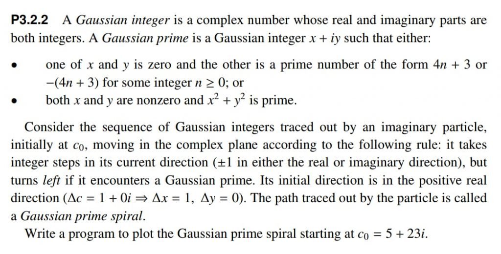
Although, history is far richer than just solving a simple problem. If you are interested try this article: Stepping to Infinity Along Gaussian Primes by Po-Ru Loh (The American Mathematical Monthly, vol-114, No. 2, Feb 2007, pp. 142-151). But here, we will just focus on the problem. Maybe in the future, I will explain this article in some video.
The plot of the path will be like this:

Beautiful!! Isn't it? Before seeing the code, let's try to understand how to draw this by hand. Let's take the initial point as $c_0=3+2i$ and $\Delta c = 1+0i=1$.
The list of all the complex number we will get for this particular example is:
| Index | Complex No. | Step | Index | Complex No. | Step |
| 0 | $3+2i$ | +1 | 7 | $2+4i$ | -1 |
| 1 | $4+2i$ | +1 | 8 | $1+4i$ | -i |
| 2 | $5+2i$ | +i | 9 | $1+3i$ | -i |
| 3 | $5+3i$ | +i | 10 | $1+2i$ | +1 |
| 4 | $5+4i$ | -1 | 11 | $2+2i$ | +1 |
| 5 | $4+4i$ | -1 | 12 | $3+2i$ | +i |
| 6 | $3+4i$ | -1 | 13 | $3+3i$ | +i |
Note that although $c_{12}$ is the same as $c_0$, as it is a Gaussian prime, the next gaussian integer will be different from $c_1$. This is the case because $\Delta c$ will be different.
To plot this, just take each $c_i$ as coordinate points, and add 2 consecutive points with a line. The path created by the lines is called a Gaussian prime spiral. Here is a hand-drawn plot.

I hope now it is clear how to plot this type of spiral. You can use the same concept for Eisenstein primes, which are also a type of 2D primes to get beautiful patterns (Excercise: Try these out for Eisenstein primes, it will be a little tricky).
We can define our function to find points of the gaussian prime spiral such that it only contains as many numbers as we want. Using that, let's plot the spiral for $c_0 = 3+2i$, which only contains 30 steps.

Here is the code to generate it. Try to analyze it.
def gaussian_spiral(seed, loop_num = 1, del_c = 1, initial_con = True):#Initial condition is actually the fact
#that represnet if you want to get back to the initial number(seed) at the end.
    d = seed; gaussian_primes_y = []; gaussian_primes_x = []
    points_x = [d.real]; points_y = [d.imag]
    if initial_con:
        while True:
            seed += del_c; real = seed.real; imagi = seed.imag
            points_x.append(real); points_y.append(imagi)
            if seed == d:
                break
            if gprime(seed):
                del_c *= 1j
                gaussian_primes_x.append(real); gaussian_primes_y.append(imagi)
    else:
        for i in range(loop_num):
            seed += del_c; real = seed.real; imagi = seed.imag
            points_x.append(real); points_y.append(imagi)
            if gprime(seed):
                del_c *= 1j ;
                gaussian_primes_x.append(real); gaussian_primes_y.append(imagi)
    gauss_p = [gaussian_primes_x,gaussian_primes_y]
    return points_x, points_y, gauss_p
Using this piece of code, we can literally generate any gaussian prime spiral. Like, for the problem of the book, here is the solution code:
seed1 = 5 + 23*1j
plot_x, plot_y, primes= gaussian_spiral(seed1)
loop_no = len(plot_x)-1
plt.ylim(21,96.5)
plt.xlim(-35,35)
plt.axhline(0,color='Black');plt.axvline(0,color='Black')
plt.plot(plot_x,plot_y,label='Gaussian spiral',color='mediumblue')
plt.scatter(primes[0][0],primes[1][0],c='Black',marker='X')#starting point
plt.scatter(primes[0][1::],primes[1][1::],c='Red',marker='*',label='Gaussian primes')
plt.grid(color='purple',linestyle='--')
plt.legend(loc='best',prop={'size':6})
plt.xlabel("Re(z) ; starting point = %s and loop number = %s "%(seed1,loop_no))
plt.ylabel("Im(z)")

plt.savefig("prob_sol.png", bbox_inches = 'tight',dpi = 300)
plt.show()
A few more of these patterns are:
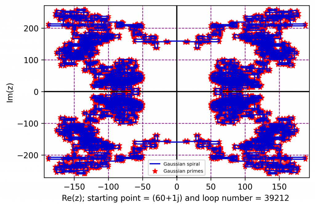
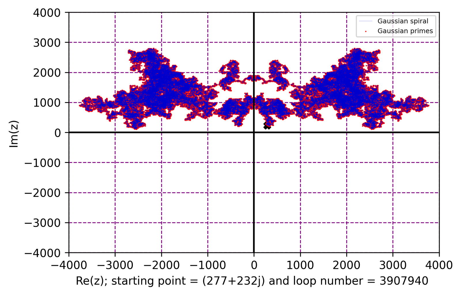
One of the most beautiful patterns is generated for the seed: $277 + 232i$.

😳 Am I seeing a Bat doing back-flip?
All the codes for generating these can be found here:
Here is an interactive version. Play around with this: https://zurl.co/Hv3U
Also, you can use python using an android app - Pydroid 3 (which is free)
I have also written this in Julia. Julia is faster than Python. Here you can find Julia's version: https://zurl.co/wETi

In 2025, 8 students from Cheenta Academy cracked the prestigious Regional Math Olympiad. In this post, we will share some of their success stories and learning strategies. The Regional Mathematics Olympiad (RMO) and the Indian National Mathematics Olympiad (INMO) are two most important mathematics contests in India.These two contests are for the students who are […]

Cheenta Academy proudly celebrates the success of 27 current and former students who qualified for the Indian Olympiad Qualifier in Mathematics (IOQM) 2025, advancing to the next stage — RMO. This accomplishment highlights their perseverance and Cheenta’s ongoing mission to nurture mathematical excellence and research-oriented learning.

Cheenta students shine at the Purple Comet Math Meet 2025 organized by Titu Andreescu and Jonathan Kanewith top national and global ranks.

Celebrate the success of Cheenta students in the Stanford Math Tournament. The Unified Vectors team achieved Top 20 in the Team Round.