An Advanced Mathematical Journey: The Structure of Operator Algebras
We are delighted to announce a new research initiative at Cheenta Academy led by Dr. Tattwamasi Amrutam, an accomplished mathematician whose work bridges deep areas of analysis and algebra.
This intensive 8-week program offers a thorough introduction to the fundamental theory of C*-algebras, a subject that bridges the worlds of analysis and algebra. Beginning with the geometric framework of Hilbert spaces, participants will explore bounded linear operators before abstracting their key properties to define C*-algebras. The course’s primary objective is to grasp the two landmark Gelfand–Naimark theorems, which demonstrate that every C*-algebra can be represented concretely—either as an algebra of continuous functions on a topological space or as an algebra of operators on a Hilbert space.
Dr. Amrutam earned his Bachelor’s degree in Mathematics and Computer Science from IMA, Bhubaneswar (2014), followed by a Master’s in Mathematics from IIT Bombay (2016). He completed his Ph.D. in Mathematics at the University of Houston in 2021 under the guidance of Dr. Mehrdad Kalantar. From 2021 to 2024, he was a postdoctoral researcher at Ben Gurion University of the Negev, working with Dr. Yair Hartman. He is currently an Adjunct Assistant Professor at the Institute of Mathematics, Polish Academy of Sciences.
Prerequisites
A strong foundation in Linear Algebra
An introductory course in Real Analysis (covering metric spaces, completeness, and continuity)
Jon the class on August 16, 2025 at 8.15PM IST as a free trial before joining the course.
Operator algebras form a unifying language for modern mathematics and physics, providing tools for understanding symmetry, quantum states, and the hidden structure of mathematical spaces. This project is designed not just to teach theory, but to develop the analytical skills and research mindset needed to engage with cutting-edge problems in pure mathematics.
Optimizing Urban Accessibility: Building a 15-Minute City with Steiner Tree Approximation
A Research Paper by Prishaa Shrimali (USA, Grade 10)
Introduction
Urban planning is increasingly focused on creating sustainable, accessible cities where essential services are within easy reach. The 15-minute city (15-MC) model is an innovative approach aimed at structuring urban spaces so that residents can access key services, like healthcare, shopping, and recreational facilities, within a short walking or biking distance. In the study Optimizing Urban Accessibility: Constructing a 15-Minute City Using Steiner Tree Approximation, researchers introduce a method of applying graph theory—particularly the Steiner tree problem—to efficiently design 15-minute cities.
Methodology
The study employs the Steiner tree problem, which seeks to find the minimum-weight network that connects selected key points, called terminals (e.g., service locations). Using this graph-based approach, the model minimizes travel time between key amenities by optimizing the pathways that connect them. Unlike models that place a focus on residential areas, this approach prioritizes service locations, making it computationally efficient.
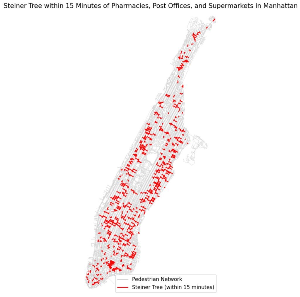
The model is applied to Manhattan, using the city's pedestrian network to highlight service accessibility. Here, amenities such as pharmacies, post offices, and supermarkets serve as the Steiner tree's focal points. The OSMnx Python library is used to pull data from Open Street Maps, allowing for a practical analysis of service accessibility within a 15-minute walking radius.
Watch the Video
Key Highlights
Efficient Service Connectivity: By focusing on connecting service points, this model minimizes computational complexity and offers a feasible layout for urban planners to improve walkability.
Dense Network Coverage in Manhattan: The analysis reveals that central and southern Manhattan already supports a high level of walkability, with the Steiner tree model indicating most residents in these areas can reach essential services within a short walk.
Areas for Improvement: The study highlights gaps in the northern parts of Manhattan, suggesting areas where pedestrian access to amenities could be enhanced.
Digital City Models: The study's approach yields detailed digital models that serve as practical tools for urban planners to optimize mobility, service placement, and sustainable design.
Inference
The Steiner tree-based method for designing a 15-minute city provides urban planners with an actionable framework to improve urban accessibility. While central areas of Manhattan demonstrate a high density of accessible services, regions like northern Manhattan could benefit from increased service points or better connectivity. This graph-based approach also shows promise for future expansions, such as multi-criteria optimization considering factors like environmental impact and cost.
In sum, the paper underscores the effectiveness of leveraging graph theory in urban planning and establishes a solid foundation for implementing sustainable, accessible city models that can adapt to the unique needs of various urban landscapes.
Collatz Conjecture and a simple program
Author: Kazi Abu Rousan
Mathematics is not yet ready for such problems.
Paul Erdos
Introduction
A problem in maths which is too tempting and seems very easy but is actually a hidden demon is this Collatz Conjecture. This problems seems so easy that it you will be tempted, but remember it is infamous for eating up your time without giving you anything. This problem is so hard that most mathematicians doesn't want to even try it, but to our surprise it is actually very easy to understand. In this article our main goal is to understand the scheme of this conjecture and how can we write a code to apply this algorithm to any number again and again.
Note: If you are curious, the featured image is actually a visual representation of this collatz conjecture \ $3n+1$ conjecture. You can find the code here.
Statement and Some Examples
The statement of this conjecture can be given like this:
Suppose, we have any random positive integer $n$, we now use two operations:
If the number n is even, divide it by $2$.
If the number is odd, triple it and add $1$.
Mathematically, we can write it like this:
$f(n) = \frac{n}{2}$ if $n \equiv 0$ (mod 2)
$ f(n) = (3n+1) $ if $n \equiv 1$ (mod 2)
Now, this conjecture says that no-matter what value of n you choose, you will always get 1 at the end of this operation if you perform it again and again.
Let's take an example, suppose we take $n=12$. As $12$ is an even number, we divide it by $2$. $\frac{12}{2} = 6$, which is again even. So, we again divide it by $2$. This time we get, $\frac{6}{2} = 3$, which is odd, hence, we multiply it by 3 and add $1$, i.e., $3\times 3 + 1 = 10$, which is again even. Hence, repeating this process we get the series $5 \to 16 \to 8 \to 4 \to 2 \to 1$. Seems easy right?,
Let's take again, another number $n=19$. This one gives us $19 \to 58 \to 29 \to 88 \to 44 \to 22 \to 11 \to 34 \to 17 \to 52 \to 26 \to 13 \to 40 \to 20 \to 10 \to 5 \to 16 \to 8 \to 4 \to 2 \to 1$. Again at the end we get $1$.
This time, we get much bigger numbers. There is a nice trick to visualize the high values, the plot which we use to do this is called Hailstone Plot.
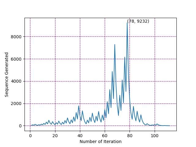
Let's take the number $n=27$. For this number, the list is $27 \to 82 \to 41 \to 124 \to 62 \to 31 \to 94 \to 47 \cdots \to 9232 \cdots$. As you can see, for this number it goes almost as high as 9232 but again it falls down to $1$. The hailstone plot for this is given below.
Hailstone for 27. The highest number and with it's iteration number is marked
So, what do you think is the conjecture holds for all number? , no one actually knows. Although, using powerful computers, we have verified this upto $2^{68}$. So, if you are looking for a counterexample, start from 300 quintillion!!
Generating the series for Collatz Conjecture for any number n using python
Let's start with coding part. We will be using numpy library.
import numpy as np
def collatz(n):
	result = np.array([n])
	while n >1:
		# print(n)
		if n%2 == 0:
			n = n/2
		else:
			n = 3*n + 1
		result = np.append(result,n)
	return result
The function above takes any number $n$ as it's argument. Then, it makes an array (think it as a box of numbers). It creates a box and then put $n$ inside it.
Then for $n>1$, it check if $n$ is even or not.
After this, if it is even then $n$ is divided by 2 and the previous value of n is replaced by $\frac{n}{2}$.
And if $n$ is odd, the it's value is replaced by $3n+1$.
For each case, we add the value of new $n$ inside our box of number. This whole process run until we have the value of $n=1$.
Finally, we have the box of all number / series of all number inside the array result.
Let's see the result for $n = 12$.
n = 12
print(collatz(n))
#The output is: [12.  6.  3. 10.  5. 16.  8.  4.  2.  1.]
You can try out the code, it will give you the result for any number $n$.
Test this function.
Hailstone Plot
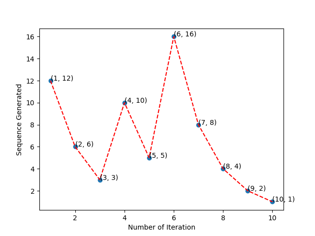
Now let's see how to plot Hailstone plot. Suppose, we have $n = 12$. In the image below, I have shown the series we get from $12$ using the algorithm.
Series and Step for $n=12$.
Now, as shown in the above image, we can assign natural numbers on each one of them as shown. So, Now we have two arraies (boxes), one with the series of numbers generated from $n$ and other one from the step number of the applied algorithm, i.e., series of natural numbers. Now, we can take elements from each series one by one and can generate pairs, i.e., two dimensional coordinates.
As shown in the above image, we can generate the coordinates using the steps as x coordinate and series a y coordinate. Now, if we plot the points, then that will give me Hailstone plot. For $n = 12$, we will get something like the image given below. Here I have simply added each dots with a red line.
The code to generate it is quite easy. We will be using matplotlib. We will just simply plot it and will mark the highest value along with it's corresponding step.
import numpy as np
import matplotlib.pyplot as plt
def collatz(n):
result = np.array([n])
while n >1:
# print(n)
if n%2 == 0:
n = n/2
else:
n = 3*n + 1
result = np.append(result,n)
return result
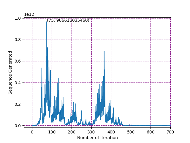
n = 63728127
y_vals = collatz(n); x_vals = np.arange(1,len(y_vals)+1)
plt.plot(x_vals,y_vals)
x_val_max = np.where(y_vals == max(y_vals))[0][0]+1
plt.text(x_val_max, max(y_vals), '({}, {})'.format(x_val_max, int(max(y_vals))))
plt.grid(color='purple',linestyle='--')
plt.ylabel("Sequence Generated")
plt.xlabel("Number of Iteration")
plt.show()
The output image is given below.
Crazy right?, you can try it out. It's almost feels like some sort of physics thing right!, for some it seems like stock market.
This is all for today. In it's part-2, we will go into much more detail. I hope you have learn something new.
Maybe in the part-2, we will see how to create pattern similar to this using collatz conjecture.
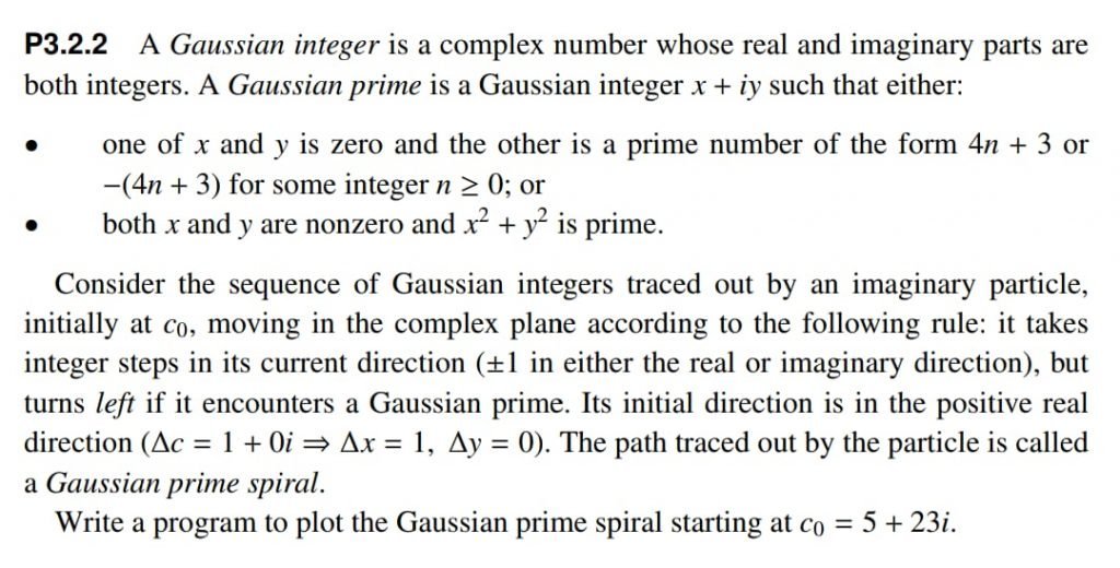
Gaussian Prime Spiral and Its beautiful Patterns
Author: Kazi Abu Rousan
Mathematics is the science of patterns, and nature exploits just about every pattern that there is.
Ian Stewart
Introduction
If you are a math enthusiastic, then you must have seen many mysterious patterns of Prime numbers. They are really great but today, we will explore beautiful patterns of a special type of 2-dimensional primes, called Gaussian Primes. We will focus on a very special pattern of these primes, called the Gaussian Prime Spiral. First, we have understood what those primes are. The main purpose of this article is to show you guys how to utilize programming to analyze beautiful patterns of mathematics. So, I have not given any proof, rather we will only focus on the visualization part.
Gaussian Integers and Primes
We all know about complex numbers right? They are the number of form $z=a+bi$, were $i$ = $\sqrt{-1}$. They simply represent points in our good old coordinate plane. Like $z=a+bi$ represent the point $(a,b)$. This means every point on a 2d graph paper can be represented by a Complex number.
In python, we write $i$ = $\sqrt{-1}$ as $1j$. So, we can write any complex number $z$ = $2 + 3i$ as $z$ = $2+1j*3$. As an example, see the piece of code below.
z = 2 + 1j*3print(z)
#output is (2+3j)
print(type(z))
#output is <class 'complex'>
#To verify that it indeed gives us complex number, we can see it by product law.
z1 = 2 + 1j*3z2 = 5 + 1j*2print(z1*z2)
#output is (4+19j)
To access the real and imaginary components individually, we use the real and imag command. Hence, z.real will give us 2 and z.imag will give us 3. We can use abs command to find the absolute value of any complex number, i.e., abs(z) = $\sqrt{a^2+b^2} = \sqrt{2^2+1^2}= \sqrt{5}$. Here is the example code.
print(z.real)
#Output is 2.0
print(z.imag)
#output is 3.0
print(abs(z))
#Output is 3.605551275463989
If lattice points, i.e., points with integer coordinates (eg, (2,3), (6,13),... etc) on the coordinate plane (like the graph paper you use in your class) are represented as complex numbers, then they are called Gaussian Integers. Like we can write (2,3) as $2+3i$. So, $2+3i$ is a Gaussian Integer.
Gaussian Primes are almost same in $\mathbb{Z}[i]$ as ordinary primes are in $\mathbb{Z_{+}}$, i.e., Gaussian Primes are complex numbers that cannot be further factorized in the field of complex numbers. As an example, $5+3i$ can be factorised as $(1+i)(3-2i)$. So, It is not a gaussian prime. But $3-2i$ is a Gaussian prime as it cannot be further factorized. Likewise, 5 can be factorised as $(2+i)(2-i)$. So it is not a gaussian prime. But we cannot factorize 3. Hence, $3+0i$ is a gaussian prime.
Note: Like, 1 is not a prime in the field of positive Integers, $i$ and also $1$ are not gaussian prime in the field of complex numbers. Also, you can define what a Gaussian Prime is, using the 2 condition given below (which we have used to check if any $a+ib$ is a gaussian prime or not).
Checking if a number is Gaussian prime or not
Now, the question is, How can you check if any given Gaussian Integer is prime or not? Well, you can use try and error. But it's not that great. So, to find if a complex number is gaussian prime or not, we will take the help of Fermat's two-square theorem.
A complex number $z = a + bi$ is a Gaussian prime, if:. As an example, $5+0i$ is not a gaussian prime as although its imaginary component is zero, its real component is not of the form $4n+3$. But $3i$ is a Gaussian prime, as its real component is zero but the imaginary component, 3 is a prime of the form $4n+3$.
One of $|a|$ or $|b|$ is zero and the other one is a prime number of form $4n+3$ for some integer $n\geq 0$. As an example, $5+0i$ is a gaussian prime as although it's imaginary component is zero, it's real component is not of the form $4n+3$. But $3i$ is a gaussian prime, as it's real component is zero and imaginary component, 3 is a prime of form $4n+3$.
If both a and b are non-zero and $(abs(z))^2=a^2+b^2$ is a prime. This prime will be of the form $4n+1$.
Using this simple idea, we can write a python code to check if any given Gaussian integer is Gaussian prime or not. But before that, I should mention that we are going to use 2 libraries of python:
matplotlib $\to$ This one helps us to plot different plots to visualize data. We will use one of it's subpackage (pyplot).
sympy $\to$ This will help us to find if any number is prime or not. You can actually define that yourself too. But here we are interested in gaussian primes, so we will take the function to check prime as granted.
So, the function to check if any number is gaussian prime or not is,
import numpy as np
import matplotlib.pyplot as plt
from sympy import isprimedef gprime(z):#check if z is gaussian prime or not, return true or false
re = int(abs(z.real)); im = int(abs(z.imag))
if re == 0 and im == 0:
return False
d = (re**2+im**2)
if re != 0 and im != 0:
return isprime(d)
if re == 0 or im == 0:
abs_val = int(abs(z))
if abs_val % 4 == 3:
return isprime(abs_val)
else:
return False
Let's test this function.
print(gprime(1j*3))
#output is True
print(gprime(5))
#output is False
print(gprime(4+1j*5))
#output is True
Let's now plot all the Gaussian primes within a radius of 100. There are many ways to do this, we can first define a function that returns a list containing all Gaussian primes within the radius n, i.e., Gaussian primes, whose absolute value is less than or equals to n. The code can be written like this (exercise: Try to increase the efficiency).
def gaussian_prime_inrange(n):
    gauss_pri = []
    for a in range(-n,n+1):
        for b in range(-n,n+1):
            gaussian_int = a + 1j*b
            if gprime(gaussian_int):
                gauss_pri.append(gaussian_int)
    return gauss_pri
Now, we can create a list containing all Gaussian primes in the range of 100.
To plot all these points, we need to separate the real and imaginary parts. This can be done using the following code.
gaussian_p_real = [x.real for x in gaussain_pri_array]
gaussian_p_imag = [x.imag for x in gaussain_pri_array]
The code to plot this is here (exercise: Play around with parameters to generate a beautiful plot).
plt.axhline(0,color='Black');plt.axvline(0,color='Black') # Draw re and im axis
plt.scatter(gaussian_p_real,gaussian_p_imag,color='red',s=0.4)
plt.xlabel("Re(z)")
plt.ylabel("Im(z)")
plt.title("Gaussian Primes")
plt.savefig("gauss_prime.png", bbox_inches = 'tight',dpi = 300)
plt.show()
Look closely, you can find a pattern... maybe try plotting some more primes
Gaussian Prime Spiral
Now, we are ready to plot the Gaussian prime spiral. I have come across these spirals while reading the book Learning Scientific Programming with Python, 2nd edition, written by Christian Hill. There is a particular problem, which is:
Although, history is far richer than just solving a simple problem. If you are interested try this article: Stepping to Infinity Along Gaussian Primes by Po-Ru Loh (The American Mathematical Monthly, vol-114, No. 2, Feb 2007, pp. 142-151). But here, we will just focus on the problem. Maybe in the future, I will explain this article in some video.
The plot of the path will be like this:
Beautiful!! Isn't it? Before seeing the code, let's try to understand how to draw this by hand. Let's take the initial point as $c_0=3+2i$ and $\Delta c = 1+0i=1$.
For the first step, we don't care if $c_0$ is gaussian prime or not. We just add the step with it, i.e., we add $\Delta c$ with $c_0$. For our case it will give us $c_1=(3+2i)+1=4+2i$.
Then, we check if $c_1$ is a gaussian prime or not. In our case, $c_1=4+2i$ is not a gaussian prime. So, we repeat step-1(i.e., add $\Delta c$ with it). This gives us $c_2=5+2i$. Again we check if $c_2$ is gaussian prime or not. In this case, $c_2$ is a gaussian prime. So, now we have to rotate the direction $90^{\circ}$ towards the left,i.e., anti-clockwise. In complex plane, it is very easy. Just multiply the $\Delta c$ by $i = \sqrt{-1}$ and that will be our new $\Delta c$. For our example, $c_3$ = $c_2+\Delta c$ = $5+2i+(1+0i)\cdot i$ = $5+3i$.
From here, again we follow step-2, until we get the point from where we started with the same $\Delta c$ or you can do it for your required step.
The list of all the complex number we will get for this particular example is:
Index
Complex No.
Step
Index
Complex No.
Step
0
$3+2i$
+1
7
$2+4i$
-1
1
$4+2i$
+1
8
$1+4i$
-i
2
$5+2i$
+i
9
$1+3i$
-i
3
$5+3i$
+i
10
$1+2i$
+1
4
$5+4i$
-1
11
$2+2i$
+1
5
$4+4i$
-1
12
$3+2i$
+i
6
$3+4i$
-1
13
$3+3i$
+i
Complex numbers and $\Delta c$'s along Gaussian prime spiral
Note that although $c_{12}$ is the same as $c_0$, as it is a Gaussian prime, the next gaussian integer will be different from $c_1$. This is the case because $\Delta c$ will be different.
To plot this, just take each $c_i$ as coordinate points, and add 2 consecutive points with a line. The path created by the lines is called a Gaussian prime spiral. Here is a hand-drawn plot.
I hope now it is clear how to plot this type of spiral. You can use the same concept for Eisenstein primes, which are also a type of 2D primes to get beautiful patterns (Excercise: Try these out for Eisenstein primes, it will be a little tricky).
We can define our function to find points of the gaussian prime spiral such that it only contains as many numbers as we want. Using that, let's plot the spiral for $c_0 = 3+2i$, which only contains 30 steps.
Here is the code to generate it. Try to analyze it.
def gaussian_spiral(seed, loop_num = 1, del_c = 1, initial_con = True):#Initial condition is actually the fact
#that represnet if you want to get back to the initial number(seed) at the end.
    d = seed; gaussian_primes_y = []; gaussian_primes_x = []
    points_x = [d.real]; points_y = [d.imag]
    if initial_con:
        while True:
            seed += del_c; real = seed.real; imagi = seed.imag
            points_x.append(real); points_y.append(imagi)
            if seed == d:
                break
            if gprime(seed):
                del_c *= 1j
                gaussian_primes_x.append(real); gaussian_primes_y.append(imagi)
    else:
        for i in range(loop_num):
            seed += del_c; real = seed.real; imagi = seed.imag
            points_x.append(real); points_y.append(imagi)
            if gprime(seed):
                del_c *= 1j ;
                gaussian_primes_x.append(real); gaussian_primes_y.append(imagi)
    gauss_p = [gaussian_primes_x,gaussian_primes_y]
    return points_x, points_y, gauss_p
Using this piece of code, we can literally generate any gaussian prime spiral. Like, for the problem of the book, here is the solution code:
The numbers 18 and 30 together looks like a chair.
The Natural Geometry of Natural Numbers is something that is never advertised, rarely talked about. Just feel how they feel!
Let's revise some ideas and concepts to understand the natural numbers more deeply.
We know by Unique Prime Factorization Theorem that every natural number can be uniquely represented by the product of primes.
So, a natural number is entirely known by the primes and their powers dividing it.
Also if you think carefully the entire information of a natural number is also entirely contained in the set of all of its divisors as every natural number has a unique set of divisors apart from itself.
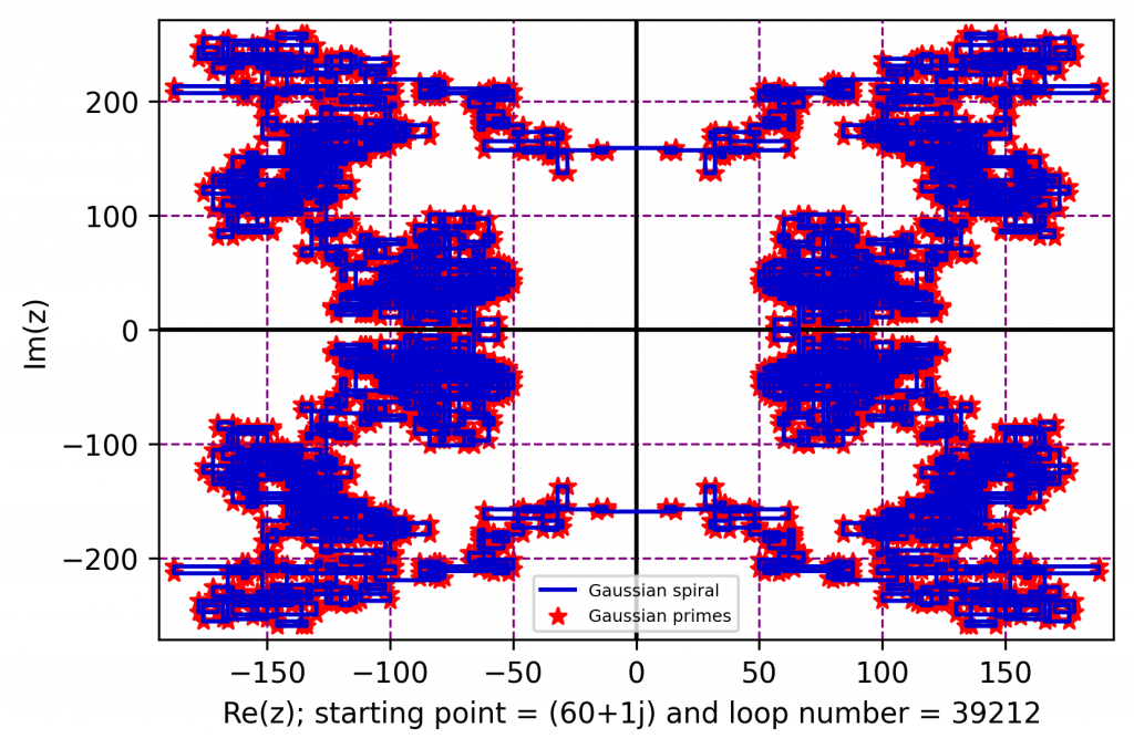
We will discover the geometry of a natural number by adding lines between these divisors to form some shape and we call that the natural geometry corresponding to the number.
Let's start discovering by playing a game.
Take a natural number n and all its divisors including itself.
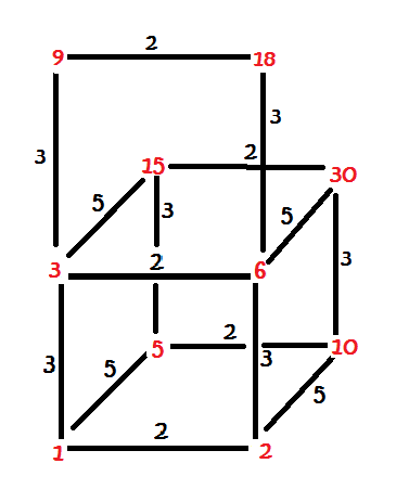
Consider two divisors a < b of n. Now draw a line segment between a and b based on the following rules:
a divides b.
There is no divisor c of n, such that a < c < b and a divides c and c divides b.
Also write the number \(\frac{b}{a}\) over the line segment joining a and b.
Let's draw for number 6.
Number 6 has the shape like a square
Now, whatever shape we get, we call it the natural geometry of that particular number. Here we call that 6 has a natural geometry of a square or a rectangle. I prefer to call it a square because we all love symmetry.
What about all the numbers? Isn't interesting to know the geometry of all the natural numbers?
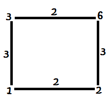
Let's draw for some other number say 30.
The Natural Geometry of 30 - A Cube
Observe this carefully, 30 has a complicated structure if seen in two dimensions but its natural geometrical structure is actually like a cube right?
The red numbers denote the divisors and the black numbers denote the numbers to be written on the line segment.
Beautiful right!
Have you observed something interesting?
The numbers on the line segments are always primes.
Actually, it shows that to build this shape the requirement of the line segments is as important as the prime numbers to build the number.
Exercise: Prove from the rules of the game that the numbers on the line segment always correspond to prime numbers.
Did you observe this?
In the pictures above, the parallel lines have the same prime number on it.
Exercise: Prove that the numbers corresponding to the parallel lines always have the same prime number on it.
Actually each prime number corresponds to a different direction. If you draw it perpendicularly we get the natural geometry of the number.
Let's observe the geometry of other numbers.
Try to draw the geometry of the number 210. It will look like the following:
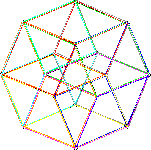
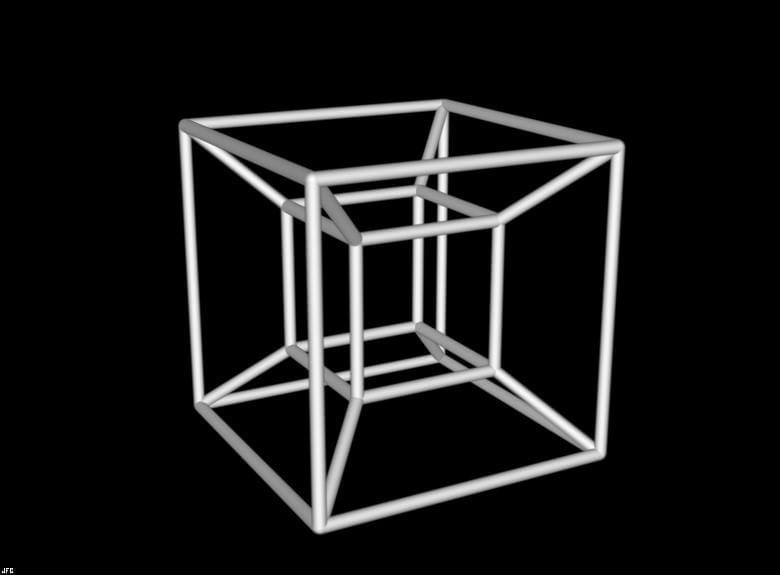
The natural geometry of the number 210 - Tesseract
This is the three dimensional projection of the structure of the Tesseract.
Obviously, this is not the natural geometry as shown. But neither we can visualize it. The number 210 lies in four dimensions. If you try to discover this structure, you will find that it has four different directions corresponding to four different primes dividing it. Also, you will see that it is actually a four-dimensional cube, which is called a tesseract. What you see above is a two dimensional projection of the tesseract, we call it a graph.
A person acquainted with graph theory can understand that the graph of a number is always k- regular where k is the number of primes dividing the number.
Now it's time for you to discover more about the geometry of all the numbers.
I leave some exercises to help you along the way.
Exercise: Show that the natural geometry of \(p^k\) is a long straight line consisting of k small straight lines, where p is a prime number and k is a natural number.
Exercise: Show that all the numbers of the form \(p.q\) where p and q are two distinct prime numbers always have the natural geometry of a square.
Exercise: Show that all the numbers of the form \(p.q.r\) where p, q and r are three distinct prime numbers always have the natural geometry of a cube.
Research Exercise: Find the natural geometry of the numbers of the form \(p^2.q\) where p and q are two distinct prime numbers. Also, try to generalize and predict the geometry of \(p^k.q\) where k is any natural number.
Research Exercise: Find the natural geometry of \(p^a.q^b.r^c\) where p, q, and r are three distinct prime numbers and a,b and c are natural numbers.
Let's end with the discussion with the geometry of {18, 30}. First let us define what I mean by it.
We define the natural geometry of two natural numbers quite naturally as a natural extension from that of a single number.
Take two natural numbers a and b. Consider the divisors of both a and b and follow the rules of the game on the set of divisors of both a and b. The shape that we get is called the natural geometry of {a, b}.
You can try it yourself and find out that the natural geometry of {18, 30} looks like the following:
Looks like a chair indeed!
Sit on this chair, grab a cup of coffee and set off to discover.
The numbers are eagerly waiting for your comments. 🙂
Please mention your observations and ideas and the proofs of the exercises in the comments section. Also think about what type of different shapes can we get from the numbers.