We are here with the Part 3 of the Arithmetical Dynamics Series. Let's get started....
Arithmetical dynamics is the combination of dynamical systems and number theory in mathematics.
Theory:
Let \( \{ \zeta_1 , ......., \zeta_m \} \) be a ratinally indifferent cycle for R and let the multiplier of \( R^m \) at each point of the cycle be \( exp \frac {2 \pi i r}{q} \) where \( (r,q) =1 \) . Then \( \exists \ k \in Z \) and\( mkq \) distinct component \( F_1 , F_2 , ..... , F_{mkq} \) s.t. at each \( \zeta_j \) there are exactly \( kq \) of these component containing a petal of angle \( \frac {2 \pi}{kq} \ at \ \zeta \) .
Further R acts as a permutation J on \( F_1 , F_2 , ..... , F_{mkq} \) where J is a composition of k disjoint cycles of length mqJ a petal based at \( \zeta_j \) maps under R to a petal based at \( \zeta_{j+1} \)
Petal theorem :
As there are \( K_j \) such cycles of components for the rationally indifferent cycle \( c_j \) , we see that there are at least \( \sum_{j} \) critical points of P in \( C \) thus \( \sum k_j \leq d-1 \Rightarrow \) we can take the uppper bound to be \( N(d-1) \)
Make sure you visit the Arithmetical Dynamics Part 2 post of this Series before the Arithmetical Dynamics Part 3.
Arithmetical Dynamics: Part 2
We are here with the Part 2 of the Arithmetical Dynamics Series. Let's get started....
Arithmetical dynamics is the combination of dynamical systems and number theory in mathematics.
The lower bound calculation is easy .
But for the upper bound , observe that each \( z \in K \) lies in some cycle of length m(z) and we these cycles by \( C_1 , C_2 .....,C_q \) . Further , we denote the length of the cycle by \( m_j \) , so , if \( z \in C_j \) then , \( m(z)= m_j \) $$ \sum_{j=1}^{q} \sum_{z \in C_j} [\mu(N,z) - \mu(m_j ,z)] $$ we can confine our attention xparatly .
Now , \( \mu(N,z) = \mu(m_j -, z) \) whenever \( z \in C_j \rightarrow \) rationally indifferent .
So , nonzero contribution comes from rationally different cycles , \( C_j \) .
Theorem:
If m|n , then \( R^n \) has no fixed at \( \zeta_j \) .
If m|n but \( m_q \not | n \) , then \( R^n \) has our fixed point at \( \zeta \) .
If \( m_q |n \) then \( R^n \) has fixed point .
Make sure you visit the Arithmetical Dynamics Part 1 post of this Series before the Arithmetical Dynamics Part 2.
Arithmetical Dynamics: Part 1
We are here with the Part 1 of the Arithmetical Dynamics Series. Let's get started....
Arithmetical dynamics is the combination of dynamical systems and number theory in mathematics.
Definition:
Suppose that \( \zeta \in C \) is a fixed point of an analytic function \( f \) .
Then \( \zeta \) is :
a) Super attracting if \( f^{'} (\zeta) =0 \rightarrow \) critical point of \( f \)
b) Attractting if \( 0 < |f^{'}( \zeta )|< 1 \ \rightarrow \) not a critical point of \( f \)
c) Repelling if \( |f^{'}( \zeta )|>1 \)
d)Rationally indifferent if \( f^{'}( \zeta ) \) is a root of unity .
e) Irratinally indifferent if \( |f^{' }( \zeta)|=1 \) , but \( f^{'}( \zeta ) \) is not a root of unity .
R has a period n ; \( R ^ {n} ( \zeta ) = \zeta \) .
If we denote \( R^m(\zeta) = \zeta-m ; m= 0, 1 ,2 ,3 ....... \) .
So $$ \zeta_{m+n}= \zeta_m \ then \ \ (R^n)^{'}( \zeta )= \prod_{i=0}^{n-1} ( \zeta_k ) \ [fixed] $$
So , we can say about attractuing , sup-attracting , repelling of \( R^n \) in terms of multiplier of \( R^n \) .
(Super)attracting points (cycles) relate to Faton set .
Today, we are going to discuss two possible problems for Arithmetical Dynamics in this post.
1.1. Existence of (pre)Periodic Points. These are the topics expanding on I.N. Baker’s theorem. Related reading:
(1) Silverman Arithmetic of Dynamical Systems: p 165. Bifurcation polynomials. Exercise 4.12 outlines some known properties and open questions (** = open question).
(2) Patrick Morton: Arithmetic properties of periodic points of quadratic maps, II – article describes where there is collapse for the family of quadratic polynomials
(3) Vivaldi and Morton: Bifurcations and discriminants for polynomial maps
(4) Hagihara - Quadratic rational maps lacking period 2 orbits
(5) John Doyle https://arxiv.org/abs/1501.06821 – a related topic but not quite the same
(6) https://arxiv.org/abs/1703.04172 – perhaps related to the question in characteristic p > 0.
(7) On fixed points of rational self-maps of complex projective plane - Ivashkovich http: //arxiv.org/abs/0911.5084 Its the only goal is to provide examples of rational selfmaps of complex projective plane of any given degree without (holomorphic) fixed points. This makes a contrast with the situation in one dimension.
Some possible questions:
(1) Is there a lower bound on the number of minimal periodic points of period n in terms of the degree of the map?
(2) What about Morton’s criteria for using generalized dynatomic polynomials (i.e., preperiodic points)? i.e., find a polynomial which vanishes at the c values where there is collapse of (m, n) periodic points.
(3) What existence of periodic points for fields with characteristic p > 0? (such as finite fields, or p-adic fields)
(4) In higher dimensions, are there always periodic points of every period? See Ivashkovich. What about morphisms versus rational maps?
1.2. Automorphisms. Readings
(1) deFaria-Hutz : classification/compuation of automorphism groups (https://arxiv. org/abs/1509.06670)
(2) Manes-Silverman arxiv:1607.05772 classification of degree 2 in P 2 with automorphisms and states a number of other open questions in Section 3 that seem tractable.
1 Possible questions: I will have a group of undergrads working on automorphism related questions this summer, so we’ll need to see what they do or do not answer (1) Dimension 1: what about existence/size of automorphim groups in characterstic p > 0. Faber https://arxiv.org/abs/1112.1999. There are a number of questions that could be asked similar to deFaria-Hutz in characteristic p.
(2) Classification of birational automorphism groups (See Manes-Silverman https:// arxiv.org/abs/1607.05772)
(3) Better bound on Field of Moduli degree (see Doyle-Silverman https://arxiv.org/ abs/1804.00700)
Arithmetic dynamics is a field that amalgamates two areas of mathematics, discrete dynamical systems and number theory. Classically, discrete dynamics refers to the study of the iteration of self-maps of the complex plane or real line. Arithmetic dynamics is the study of the number-theoretic properties of integer, rational, $latex p$-adic, and/or algebraic points under repeated application of a polynomial or rational function. A fundamental goal is to describe arithmetic properties in terms of underlying geometric structures.
Given an endomorphism $latex f$ on a set $latex X$; $latex f:X\to X$ a point x in X is called preperiodic point if it has finite forward orbit under iteration of $latex f$ with mathematical notation if there exist distinct n and m such that $latex f^{n}(x)=f^{m}(x)$(i.e it is eventually periodic''). We are trying to classify for which maps are there not as many preperiodic points as their should be in dimension $latex 1$. It is a more precise version of I.N. Baker's theorem which statesLet $ $latex P$ be a polynomial of degree at least two and suppose that $latex P$ has no periodic points of period $latex n$. Then $latex n=2$ and $latex P$ is conjugate to $latex z^2-z$.''
Research in Arithmetical Dynamics: Steps
The hurdles that we have to cross to do some research on Arithmetical Dynamics is:
Group Theory (Dummit and Foote)
Commutative algebra( Atiyah, Mcdonald)
Algebraic Number Theory (Marcus)
Algebraic Geometry (Shafarevich)
Dynamical System (Silverman)
Chaos ... at Cheenta!
CHAOS ... Starting 15th August, 8 PM at Cheenta. Be online on Skype (if you are added to Cheenta Open Slate)
An Introduction to Chaos
The concept of chaotic systems goes back to Newtonian mechanics, but the current qualitative approach began only in the late 1800s. In this talk, we shall try to explain informally the concept, give some simple examples and introduce some of the tools used to study them.
Prerequisites: Single variable calculus
Faculty: Sankhadip Chakraborty, (Chennai Mathematical Institute, IMPA Brazil; Pursuing Ph.D. in Dynamical Systems)
Research Track Day 1 Group Theory
Group Theory
Group Theory is the study of groups in mathematics and abstract algebra.
This is an excerpt from Cheenta Research Track training burst.Research Track program has two components.
Training burst (a sequence of 3/4 sessions to help students acquire necessary background knowledge). This may happen in certain months of the year.
Weekly / biweekly meetings (to work on a specific problem)
Group
Group is a collection of ‘forces’ that can move points in a space. (This is not definition of a group, just a way to think about it). Understanding the ‘action’ of a group on a ‘space’ helps us to understand the group better.
Groups are usually big (containing infinitely many elements). We want to break it down into smaller blocks. This is similar to factorization of large numbers into prime factors. In fact, it is a common theme all across life: see a big problem? Break it down into small, manageable parts and try to understand the parts.
How do we factorize groups?
One way is to understand group action on a space. We won’t give definitions here. Rather, we will give examples.
First example
Consider the group of integers: {0, 1, -1, 2, -2 .. }
Why is this set a group? It satisfies the four conditions that make a set a group:
Add any two and you will get a third element of the set (hence set of odd numbers is not a group. )
There is an identity element (the do-nothing element). In this set it is 0. Add it to any other element a. You will get a back.
Each number has inverse — the undo operation. For example element 2 has an inverse: -2
addition is associative
Next consider the space of real line (\( \mathbb{R}\). It is the set of real numbers.
Finally consider the action of G (group) on the S (space). Here is the catch - point. You have to image each group element as a force which can potentially move a point in the space using a certain rule.
There can be many rules. We are interested in some. They should have a couple of desirable properties:
The do-nothing element of the group (identity element) should literally be the 0-force and not move any element of the space at all.
If \( g_1, g_2 \) be two forces and P be a point in the space. Suppose applying the force \( g_1 \) to P it moves to Q. Then applying \(g_2\) to Q, it goes to R. But the action is such that you are allowed to do a different thing: combine the forces \(g_2, g_1\) inside the group and then apply the resulting force to P and you will reach R.
If you know the basic definition of group action, even then it helps to think about it in this way.
Group Theory Action
What will the force 2 do to the point 5.3?
It may send 5.3 —> 7.3. It may send 5.3 —> 3.3. We can define other weird rules as well. For example \( 5.3 —> 5.3^2 \). Somehow we have to use the numbers 5.3 and 2 and think about 5.3 as a point on the line and 2 as a force.
If the rule is translate to the right then we get the circle from the line! This was discussed in the very last section of this session (fundamental group).
Groups acting on trees (notes from Cheenta Research Track)
Groups can be very complicated. One way to understand complicated objects is to break them into simpler pieces. For example, to understand large numbers, we often factorize them into their prime constituents.
How do we 'factorize' groups?
Instead of looking at the group, we try to examine how it 'acts' on some space. Imagine the group elements as 'strikers' and points in the space as 'balls'. When the group elements (strikers) acts on (hits) the points in the space (balls), the balls may move a bit. We examine the movement of the balls to factorize the group!
How?
Let's work with a specific type of space: two dots connected with a segment.
Suppose a group G is acting on this space T.
(We are speaking very loosely here. We have not defined what is meant by group action. For the moment, the striker-ball analogy should suffice).
A chunk of the group G may 'fix' portion of this interval. Let us call this chunk H. H will be treated as a factor of the group G.
Next we will look at the endpoints of this interval. Some chunks larger than H (and containing H) could fix the endpoints. These will give further factorization of the group.
Notice that we are using the words 'could' and 'may'. This is deliberate. Whether or not this will happen, will depend on the group under examination.
This is in nutshell what group action on trees is all about. It involves beautiful ideas from graph theory, topology and geometric group theory.
Research Track - Cocompact action and isotropy subgroups
In mathematics, if the quotient space X/G is a compact space, then it is called cocompact action of a group G on a topological space X. If X is locally compact, then an equivalent condition is that there is a compact subset K of X such that the image of K under the action of G covers X.
Suppose a group $latex \Gamma $ is acting properly and cocompactly on a metric space X, by isometries.
(Understand: proper, cocompact, isometric action)
Claim
There are only finitely many conjugacy classes of the isotropy subgroups in $latex \Gamma $
Sketch
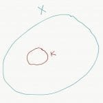
Since the action is cocompact, there is a compact set K whose translates cover X.
cocompact action
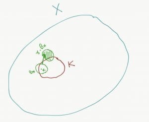
For each $latex x \in K $, choose small (enough) balls $latex B_x $.
How small do we want the balls?
Small enough, such that all but finitely many of the translates of the ball is disjoint from the ball.
In the picture, the green blob around x in K is an example of $latex B_x $ . It is small enough such that $latex \gamma \cdot B_x $ is disjoint from $latex B_x $. The ball $latex B_x $ is small enough such that most almost $latex \gamma $ this should happen (except finitely many of them).
How do we know that there is such a ball? This is by definition of proper action. Since the action is proper, by definition, we will get such balls for each x in X.
Intuitively a proper action is proper, that is, most of them (the isometries) move balls considerably.
Examples to keep in mind: Integer translation on the real line is proper. Rational translation on the real line is not proper.
$latex \cup B_x $ is an open cover of K. Hence it has a finite subcover (as K is compact).
Choose finitely many balls $latex B_{x_1}, \cdots , B_{x_k} $, such that they cover K.
These finitely many balls have two properties:
They cover K
$latex \gamma \cdot B_{x_i} \cap B_{x_i} \neq \phi $ for finitely many $latex \gamma \in \Gamma $
Thus each member of $latex \Sigma $ has this property : hit all of the balls in the previously found cover by it. At least one of them will not move a lot (that is the translate will have a non-empty intersection with the ball)
Also notice that $latex \Sigma $ is finite (as there are finitely many balls and for each ball there are finitely many $latex \gamma $.
Suppose $latex x \in X $ be any point. There is a $latex \gamma \in \Gamma $ such that $latex x \in \gamma \cdot K $.
Then $latex \gamma^{-1} \cdot x \in K $ . This is the element of K that goes to x under $latex \gamma $
cocompact action
Now consider the isotropy subgroup $latex \Gamma_x $, that is group of all isometries that fixes x.
Notice that $latex \gamma^{-1} \Gamma_x \gamma $ is the isotropy subgroup of $latex \gamma^{-1} \cdot x $. Why? Suppose $latex \gamma_1 \in \Gamma_x $. We will show that $latex \gamma^{-1} \gamma_1 \gamma ) fixes ( \gamma^-1 \cdot x $.
After all $latex \gamma^{-1} \gamma_1 \gamma ( \gamma^{-1} \cdot x) = \gamma^{-1} \cdot x $
We can similarly show the converse.
Hence we have shown that if x is pulled back into K by some $latex \gamma^{-1} $ conjugating the isotropy subgroup of x by that $latex \gamma $ gives the isotropy subgroup of the pulled back element.
But this is the subgroup that does not move the ball in the cover containing $latex \gamma^{-1} \cdot x $ in a disjoint manner. Hence it must be inside $latex \Sigma $, and hence finite as $latex \Sigma $ was finite.