‘Proper’ is a heavily overloaded term, both in life and in mathematics. It may mean different stuff in different contexts. Thankfully mathematics is far less complicated that life and we can rigorously define properness.

Proper Function: A continuous function ( f : X  \to Y ) between topological spaces is proper if the preimage of each compact subset of Y is compact.

Proper Space: A metric space (X, d) is proper if every closed ball ( B[x, r] = { y \in X | d(x, y) \leq r } ) in X is compact.

Intuition: Proper Spaces have much in common with Euclidean Spaces. Why? Heine Borel Theorem ensures that, closed balls are compact in Euclidean Space. Proper Spaces own this property as well.

There is a fancy description of Proper Spaces using Proper Functions.

Also see

College Mathematics Program at Cheenta

Theorem:

Let (x_0 ) be an element of the metric space (X, d) and define ( d_0 : X \to [0,\infty) by d_0 (x) = d(x_0, x) ) . Then (X, d) is proper iff ( d_0 ) is proper.

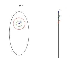
We will rigorously prove this theorem. But first, lets draw some pictures.

Driving Idea: Which points in X map to the point ( a \in [0, \infty) ) ? They must be the points which are a distance away from ( x_0 ). Hence they are circles in X centered at ( x_0 ).

Proof:

(It is useful to try and write your own proofs first)

—> Suppose \( d_0 \) is a proper map. Then we will show that (X, d) is a proper space (that is all closed balls are compact).

Consider the compact set [0, a] (a is a finite number) in ( [0, \infty) ). This is a compact set (in ( [0, \infty) ).

Then its inverse image ( d_0^{-1} ([0, a) ) ) is compact in (X, d). (This is true because we have assumed (d_0 ) is a proper map, hence inverse images of compact sets will be compact).

But ( d_0^{-1} ([0, a) ) ) is a closed ball centered at ( x_0 ) of radius a. Thus we showed that all closed balls centered at ( x_0 ) are compact.

Next we will show that any other closed ball is compact. Consider a closed ball B of radius r, centered at ( x_1 \in X ). Suppose ( d(x_0, x_1) = t ) We take the ball B’ of radius t + r centered at ( x_0 ).

If ( x \in B ) then ( d (x , x_1 ) \leq r ). Next we use the triangle inequality to compute:

$$ d(x_0, x) \leq d(x_0, x_1) + d(x_1, x) \leq t + r $$

Hence x is in ball B’ centered at ( x_0 ) . Therefore B is contained in B’.

Suppose ( { U_{\alpha} }{\alpha \in \Lambda}  ) is an arbitrary open cover of B (the closed ball centered at (x_1) ). Since B is closed (by assumption), therefore ( B^c ) is open and ( { { U{\alpha} }_{\alpha \in \Lambda} , B^c } ) is an open cover for B’.

Earlier we showed that all closed balls centered at ( x_0 ) are compact. B’ is one such balls. Hence it is compact. Hence ( { { U_{\alpha} }_{\alpha \in \Lambda} , B^c } ) has a finite subcover that covers B’. Since B is inside B’, this finite subcover also works for B’. If necessary, by removing ( B^c ), we get a finite subcover of B. Hence B is compact.

<—- Suppose (X, d) is proper. Then we will show that \( d_0 \) is a proper map.

Suppose V is a compact subset of ( [0, \infty ) ). By Heine Borel Theorem, it is closed (contains all its limit points) and bounded. Since V is bounded, it has an upper bound. By Completeness axiom, it has a least upper bound L. Since it is closed, this least upper bound L is inside V.

( d_0^{-1} (L)  ) is the circle of radius L centered at ( x_0 ). Every other point in the pre-image of V, is on a circle centered at ( x_0 ) of radius less than or equal to L. Hence the pre-image of V is bounded.

We will show that every infinite sequence has a convergent subsequence (sequential definition of compactness).

Suppose ( < x_n > ) is an infinite sequence in the pre image of V. Then ( d_0 ( x_n ) = a_n ) is an infinite sequence in V. As V is compact, it has a convergent subsequence (d_0 (x_{n_k}) = a_{n_k}) that converges to some ( a \in  V ).

The preimage of a under (d_0 ), is the collection of all points from ( x_0 ) at a distance away. The distance from ( < x_{n_k} > ) to (B [x_0 , a] ) is 0 as ( d (x_{n_k} , x_0) ) approaches a as (n_k \to \infty ). If no point on ( \partial B ) (boundary of the ball) is a limit point of the sequence, then we can build an open cover using open balls ( U_x ) at each point on the boundary that completely misses the sequence (< x_{n_k} > ) and int (B).

Since ( B[x, a]) is compact, this open cover has a finite subcover. Let ( int (B), U_{x_1} ,  ... , U_{x_n} ) be the finite subcover. This leads to a contradiction as ( < x_{n_k} > ) cannot be closer to the boundary than the minimum of the distances of these finitely many open sets (each of which completely misses the sequence).

Proper Spaces share more properties with Euclidean Spaces. For example, every proper metric space is complete.

Proof:

Suppose ( < x_k> ) is Cauchy in a proper space (X, d). That is ( \forall \epsilon > 0 \exists N \in \mathbb{N} \ni \forall m, n > N, d(x_m, x_n) < \epsilon ).

This implies ( | d(x_m, x_0) - d(x_n, x_0) | < d(x_m, x_n) < \epsilon ). Therefore ( |d_0 (x_m) - d_0 (x_n) | < \epsilon ) in ( [0, \infty) ).

Hence ( d_0 ( x_k) ) is Cauchy in ( [0, \infty) ). Since ( [0, \infty) ) is complete, therefore this converges to some nonnegative number a.

Finally using arguments similar to the last part of the previous proof, we are done.

One Point Compactification

Theorem: Show that a continuous function ( f : X \to Y ) between proper metric spaces is proper iff the obvious extension ( f : X^* \to Y^* )  between one-point compactification spaces is continuous.

Proof: 

Recall One Point Compactification:

Put ( {\displaystyle X^{}=X\cup {\infty }}  ) , and topologize ( {\displaystyle X^{}}  ) by taking as open sets all the open subsets U of X together with all sets ( {\displaystyle V=(X\setminus C)\cup {\infty }}  ) where C is closed and compact in X. Here, ( {\displaystyle X\setminus C} )  denotes setminus. Note that ( {\displaystyle V} ) is an open neighborhood of ( {\displaystyle {\infty }} ), and thus, any open cover of ( {\displaystyle {\infty }} ) will contain all except a compact subset ( {\displaystyle C} ) of ( {\displaystyle X^{}} ) , implying that ( {\displaystyle X^{}} ) is compact.

Proper --> Continuous

Suppose ( f : X \to Y ) is proper. We will show that ( f^* ), the extension of f, is continuous. Toward that extent, we will show that inverse of any open set is open. Clearly if, ( V \subset X^* ) does not contain ( \infty_Y ) then its preimage is open in ( X^* ) as f is continuous.

If ( V \subset Y^* ) contains ( \infty_Y ) then( {\displaystyle V=(Y \setminus C)\cup {\infty_Y }}  ) where C is closed and compact in X. Then

( \displaystyle { {f^}^{-1} ( (Y \setminus C) \cup { \infty_Y } ) \ = { {f^}^{-1}  (Y) -  {f^}^{-1} ( C) } \cup {f^}^{-1} { \infty_Y } \ = {X - f^{-1}(C)}  \cup {\infty_X } } )

SInce f is proper ( f^{-1} (C) ) is compact and we have an open set of ( X^* ) as the preimage.

Continuous --> Proper

Suppose V is an open set in ( Y^* ) containing ( \infty_Y ). Since ( f^* ) is continuous, its preimage must be open.

( {\displaystyle V=(Y \setminus C)\cup {\infty_Y }}  ) where C is closed and compact in X

( \displaystyle { {f^}^{-1} ( (Y \setminus C) \cup { \infty_Y } ) \ = { {f^}^{-1}  (Y) -  {f^}^{-1} ( C) } \cup {f^}^{-1} { \infty_Y } \ = {X - f^{-1}(C)}  \cup {\infty_X } } )

This implies ( {X - f^{-1}(C)}  \cup {\infty_X }  ) is open in ( X^* ) containing ( \infty ). This implies ( f^{-1} (C) ) is compact (due to the characterization of open sets containing infinity). SInce for all compact subsets C of Y, the above argument is valid, therefore f is proper.