In this post, we will be discussing mainly, naive Bayes Theorem, and how Laplace, developed the same idea as Bayes, independently and his law of succession go.

I cannot conceal the fact here that in the specific application of these rules, I foresee many things happening which can cause one to badly mistaken if he does not proceed cautiously.

James Bernoulli

While watching a cricket match we often, try to predict what may happen in the next ball, and several time, we guess it correctly, I don't know much about others, but my predictions very often turns out to be true, even to the extent that, if I say, " may be Next ball will be an out-side edge caught behind by the keeper" and such thing really happens withing next 2 or 3 balls if not the immediate next ball. In college, I had a friend who could also give such precise predictions while watching a cricket match, even though he was not a student of probability. So, you see while at home or among friends, people think that we are getting lucky about our predictions.

Well, truly speaking, there's nothing wrong in that assumptions, we are indeed guessing and getting lucky. But what matters is our chance of getting lucky with our predictions is relatively higher than others !! While talking about chances, remember while making our judgements, we have no mathematical chances in our hand on which we are making predictions. What we just know is that, the proposition, we are predicting has reasonably higher probability than any other outcomes, we can think off. But how reasonable ?? Really No idea !! Actually see to take a decision regarding what may happen in the next ball, we don't need to know the mathematical probabilities, rather the need of developing probability is quite the other way around. i.e. for a judgement or proposition, you think its gonna happen or its true, we need to develop probabilistic calculation to judge how significant is my prediction.

Say, you are a manager of a cricket team(not an ordinary), and you need to pick a team for a future tournament, and you need to observe the performance in this current season, as you want to give a significant weightage on the current form of the players. So, here working with your instinctive judgements can even cost you your job. So, here you need to be sure about the relative-significance of your judgements, and take a final decision. We will come to these sort of problems, later while discussing about how decision making can be aided by Bayesian thinking. And that's where the real need of this theory lies. But as it happens, to apply first we need to our idea about the nature of these thinking quite clear. So, for now we will deal with some hypothetical but interesting problems.

Am I really Guessing ?

Well, it depends what definition of guessing you are setting. Ofcourse I was guessing, but the question is if my guesses are often correct, what is the possible explanation ?? The answer is quite simple, I'm not making judgements emotionally !! Often people realise that this may be their favorite batsman may miss a ton, but still stay emotional in predicting that !! What, parameters I always look into is the parameters where a sane probability believer will put his/her eyes on, i.e. How often, the batsman scores runs in consecutive matches, which bowler bowling and his\her ability ton swing the ball away from the batsman, in order to have an outside kiss from the bat, how often the batsman facing the ball, leaves or play balls outside off, etc etc etc. Any serious cricket lover will keep these things in account while making judgements. So, you see we are not actually guessing randomly. We are using information from every single ball. Hence, I'm always updating the chance of the propositions which I think may happen, with the information, I'm extracting after each ball is played. In precise our decision making is itself a Bayesian Robot, if and only if we are ready to give our biases !!

Naive Bayes

We have already discussed about how the seed of inverse thinking to establish possible causal explanation was planted by Thomas Bayes. (if you haven't read our previous post, here it is Bayes and The Billiard Table | Cheenta Probability Series ). The astonishing thing is that, even though Bayes' idea of evaluating inverse probability using available information was intuitive and mathematical enough, it still remained unknown or criticized if known in most of the Europe. There were mainly two reasons for that, first, may advanced thinking was not the cup of tea which the 18th century mathematicians and probability people, were ready to drink, they eventually needed the evolution of Computer to drink that cup completely, and the second reason was that, even though Bayes' idea was intuitive and radical, it needed serious mathematical support, or it would have collapsed.

So, Bayes idea was quite simple and elegant. Suppose you have a suspicion, say \(S\), say the batsman will not score a ton. Then, you have a set of information say \(I\), say that s\he scored a ton in the last match. So, the chance (or expectation) of your suspicion \(S\) to be come true, when you have observed \(I\) is the ratio of the chance (or expectation) that you had observed this kind of information \(I\), when actually your suspicion was correct and the chance of observing what you have observed i.e. chance of observing \(I\). So, mathematically,

\(P(S|I)=\frac{P(I|S)P(S)}{P(I)}\)

If we break down the \(P(I)\), using Total Probability (or expectation) law, (remember !!), then we will get the form of Bayes theorem, we are accustomed to see in our textbooks,

\(P(S|I)=\frac{P(I|S)P(S)}{P(I|S)P(S)+P(I|S^c)P(S^c)}\) .

Hence, here our Prior probability is \(P(S)\) .i,e. chance of your suspicion to be true, gets updated to the posterior probability \(P(S|I)\), i.e. chance of your suspicion to be true when you have observed some information supporting or doubting your suspicion. The point is you state about the truth of your prediction is changing towards the reality !

Now in the above, expression, the place where controversies arises, is what is the nature of \(P(S)\) ? that is how often, your (our), suspicion about a particular thing turns out to be true ? Here comes our hypothetical problem of Extrasensory Perception which we will ultimately converge in to the Law of Succession, developed by none other than the great Laplace.

Laplace Places his Thoughts

Now, suppose we are interested to know what is the chance, that my guess about the next next ball will be correct, when it is already known that some of the guesses I made earlier turned out to be correct.

Let, I, have made \(n\) guesses earlier as, \(G_1,G_2,....,G_n\) among which \(k\) guesses turned out to be correct, now if I make another guess say, \(G_{n+1}\), what is the chance that my current guess will turn out to be true ?

Now, we will present the solution to this problem, but we will first develop the the story and intuition developed by one of the pioneer of this field. The solution turned out to be a law in future.

Thoughts are often like noises, that pops-up here and there, when in England, Bayes's hidden work got published and didn't got due attention, then in other part of Europe, the similar thoughts pops-up in the mind of young but brilliant Pierre-Simon Laplace. Now obviously I don't need to say more about who he is.

That was the era when Astronomy was most quantified and respected branch of science. The Science was looking forward to test Newton's Theories by explaining how precisely gravitation effects the movements of tides, interacting planets and comets, our moon, and the shape of the Earth and other planets. Years of Empirical data was collected. The Scientists and astronomers everyday went to sleep with the fear that, a single exception in their expected data could bring the entire edifice tumbling down. The question which all mattered is whether the Universe is stable !!

Astronomers, knew the planets are moving. There came a time some of them feared that slowly accelerating Jupiter will smash into the Sun someday !! The problem of predicting the motions of many interacting bodies over long periods of time is complex even today, and Newton concluded that God's miraculous intervention kept the heavens in equilibrium.

Laplace who was an Astronomer turned mathematician, took it as a challenge to explain the stability of the Universe and decided dedicating his thoughts in that. He said that while doing this Mathematics will be his telescope in hand. For a time being, he started considering ways to modify Newtons's theory of gravitation by making gravity vary with a body's velocity as well as with its mass and distance. He also wondered fleetingly whether comets might be disturbing the orbits of Jupiter and Saturn. But he changed his mind almost immediately. He realised the problem was not Newtons Theory, but the data collected by the astronomers.

Newtons's system of Gravitation, could have been verified, only if the measurements would come precise and as expected. But observational astronomy was awash with information, some of it uncertain and inadequate. That's where Laplace felt the need to introduce probability in his scientific research. This is also a very important moment for probability theory, it came out from its gambling table and got preference on the papers of a scientist. But still Laplace was far enough from the Bayesian ideas, which he was to develop in future.

In next five years Laplace wrote 13 papers in solving problems in astronomy and mathematics of celestial mechanics but still was rejected from getting membership, in French Royal Academy of Sciences. Then a time came when he actually started considered , of emigrating to Prussia to work in their academies. During this frustrated period, when he used to spent his afternoons digging in mathematical literature in libraries. And remember he was still worried about the problem with the errors in the measured astronomical data, and was beginning to think that it would require a fundamentally new way of thinking, may be probability theory to deal with the uncertainties prevading many events and their causes. That is when he began to see the light. And in that light he found the same book, which even stimulated the grey cells of Thomas Bayes, just a decade ago, he got "The Doctrine of Chances" by Abraham de Moivre. May be Laplace studied a new version of the book, unlike Bayes.

Laplace's growing interest in probability theory created a diplomatic problem, stalwarts like d'Alembert believed probability was too subjective for developing scientific arguments. But Laplace was young and daring to bring revolution in the thinking. He was quite sure that only probability can help him in getting precise solution while dealing with the complex problems of movements in celestial bodies. And in the process he immortalized Probability Theory while finding its application in such a higher form of scientific investigations. He began thinking, how he can find an causal explanation, behind the divergence in the error filled observations. He independently developed a thought behind developing " Probability of Causes" derived from the already happened events.

In is first paper on this topic, in 1773, atheist Laplace compared ignorant mankind, not with God but with an imaginary intelligence capable of knowing it all. Because humans can never know everything with certainty, probability is the mathematical expression of our ignorance : "We owe to the frailty of the human mind one of the most delicate and ingenious of mathematical theories, namely the science of chance or probabilities."

He often said he did not believe in God, but neither her Biographer could decipher whether he was an atheist or a diest. But his probability of causes was a mathematical expression of the universe, and for the rest of his days he updated his theories about God and probability of causes as new evidence became available.

Laplace's Principle of Succession

Laplace, at first dealt with the same problem as Bayes, about judging the bias of a coin, by flipping it a number of times. But, he modified a version which was quite identical to the philosophical problem, proposed by Hume, which asks the probability that the sun going to rise tomorrow when you know that sun is being rising everyday for the past \(5000\) years. Observe that it also very much coincides with the problem of guessing I presented at the beginning of this section.

He developed his principle, which mathematically equates as the formula we came across in the Naive Bayes, infact that form of Bayes rule is more due to Laplace than due to Bayes himself !! So, using his principle, and accepting the restrictive assumption that all his possible causes or hypotheses were equally likely, he started using the Uniform prior. Laplace calculates the probability of success in the next trial ( sun rising tomorrow ), given there are \(n\) successes earlier in all \(n\) trials.

He, defined, a variable ( which we call Random Variable), \(X_i \) which takes value of \(1\), if success comes at \(i\) th trial or \(0\) if failure. Now, with what probability, a success will come that is unknown to us, and that what the unknown bias is, hence he took that chance say, \(p\) to be distributed uniformly within the interval, \((0,1)\). Let the probability density of \(p\), be \(f\). Now, let \(S_n\) be the number of success in \(n\) trials. Then, \(S_n= X_1+X_2+....+X_n\). Here, \(S_n=n\). So, we need, \(P(X_{n+1}=1 |X_1=1,X_2=1,....,X_n=1)\) which is precisely, \(P(X_{n+1}|S_n=n)\).

Laplace principle was, The probability of a cause ( success in the next trial) given an event ( past \(n\) trials all resulted in success) is proportional to the probability of the event, given the cause. Which is mathematically,

\(P(X_{n+1}=1 | S_n=n) \propto P(S_n=n|X_{n+1}=1)P(X_{n+1}=1)\)

Now, see that the event of success in next trial can occur with probability \(p\) that we don't yet know, and wish to know. So, with \(X_{n+1}=1\) we are actually claiming the chance of success is \(p\), which is uniformly distributed within \((0,1)\). So, Now the question is what a should be the constant of proportionality ?? Laplace is witty enough to answer that the constant of proportionality is nothing but the normalizing constant of the posterior probability, \(P(X_{n+1}=1 |S_n=n)\) !! Since we know, conditional probabilities are also probabilities and they also follow the conglomerability and adds up to 1. Hence, in this case, the required constant is \(\frac{1}{P(S_n=n)}\) .

Now, in our statement of proportionality becomes,

\(P(X_{n+1}=1|S_n=n)=\frac{P(S_n=n|X_{n+1}=1)P(X_{n+1}=1)}{P(S_n=n)}\). Isn't it look like the Bayes rule we all know !!

Now there are two, ways the probability can be computed, I will present the elegant and more complicated way, the other you can search yourself!!

As, I was discussing that, the event \(X{n+1}=1\) is bijective to the even that the success chance is some \(p\). So,

\(P(S_n=n|X_{n+1}=1)P(X_{n+1}=1)=P(S_n=n| success \ probability \ is p \ is \ uniform \ in \ 0<p<1 )P(X_{n+1}=1|success \ probability \ is p \ is \ uniform \ in \ 0<p<1) \\= \int^1_0 p^n p \,dp= \frac{1}{n+2}\), integrated since we consider all values within the interval \((0,1)\) has same density i.e. \(f(p)=1\) when \(0<p<1\). Now our required posterior is,

\(P(X_{n+1}=1|S_n) \propto \frac{1}{n+2}\),

Now, one can verify that, our normalizing constant, \(P(S_n=n)\) is\( \frac{1}{n+1}\). Use, Law of total probability over \(0<p<1\), using the prior density of \(p\). Hence, finally, Laplace got,

\(P(X_{n+1}=1|S_n=n)=\frac{n+1}{n+2}\). Hence the chance of the sun rising tomorrow when it has risen, past \(n\) days is \(n+1\) out of \(n+2\). Now, the solution to the guessing problem is also a matter of assessing the same arguments, which I leave in the hands of the reader, to find out. Another thing to note here, that Laplace, was the first called this conditional probability as likelihood, which became a quite important part of literature in Bayesian inference.

This principle, then went on to be known as the "Laplace Law of Succession". The rationale behind the nomenclature is, that with the information about the outcome of every trial, one can update the information about the chances of the success, in a successive order. Just like Thomas Bayes updated his information about the position of his read ball relative to the position of each black ball rolled on the billiard table.

Notice that for large numbers of trials an application of Laplace's rule is very close to simply taking the relative frequency of heads as ones's probability for heads the next time. In this setting, with a lot of data, naive frequentism does not go far wrong. But who, on initially getting two heads, would give probability one on heads the next time ?

Laplace Generalizes

Now, the controversy or may be in some cases, fallacy of this more rightfully called, Bayes-Laplace Rule, was at the uniform approximation of the priors. Suppose a flat prior is not appropriate. That is in most cases the coin may be biased, but it is unlikely to be very biased. Perhaps one might want a prior like a symmetric bell-shaped distribution,

or it may be more likely to be biased in one direction having a skewed bell-shaped prior.

Then the questions arises are, Can the simplicity and tractability of the Bayes-Laplace analysis be retained ? It can. We choose an appropriate prior density proportional to the likelihood.

As, I discussed in the solution above, Laplace, wittily used the normalizer of the posterior probability of distribution, as the constant of proportionality, which further made the prior density to integrate to \(1\).

The distribution we basically considered in the above solution could be generalized by Beta distribution, whose shapes are governed by the parameters of it that are often names as \(n\) and \(m\). The density of beta looks like,

\(\frac{p^{n-1}(1-p)^{m-1}}{normalizer} \), here, the Bayes-Laplace flat prior has both \(n\) and \(m\) equals to 1. While in the symmetric bell-shaped prior, which is peaked at \(\frac{1}{2}\), has both \(n\) and \(m\) to be equal to \(10\), whereas in the second case of the skewed prior, the \(n\) is taken to \(5\) and \(m\) kept same as \(10\).

Now, since the principle of Laplace states the prior density is proportional to the likelihood, pilling up frequency data keeps the updated density in the beta family. Suppose starting with parameters \(n\) and \(m\), in a squence of \(t\) trials, we incurred \(s\) successes. Hence, our new beta density will have parameters \(n+s\) and \(m+(t-s)\). The resulting rule of succession gives us the probability of success for the next trial, on the evidence of \(s\) successes in \(t\) trials, as \(\frac{s+n}{t+n+m}\),

Clearly as claimed at the end of the last section, this ratio almost becomes the relative frequency \(\frac{s}{t}\), for large number of trials, which again swamps the prior. How fast this swamps the prior that depends on the magnitude of \(n\) and \(m\).

This is here where we can actually look into not only the predictive power of this rule, but also how it updates its densities about the unknown.

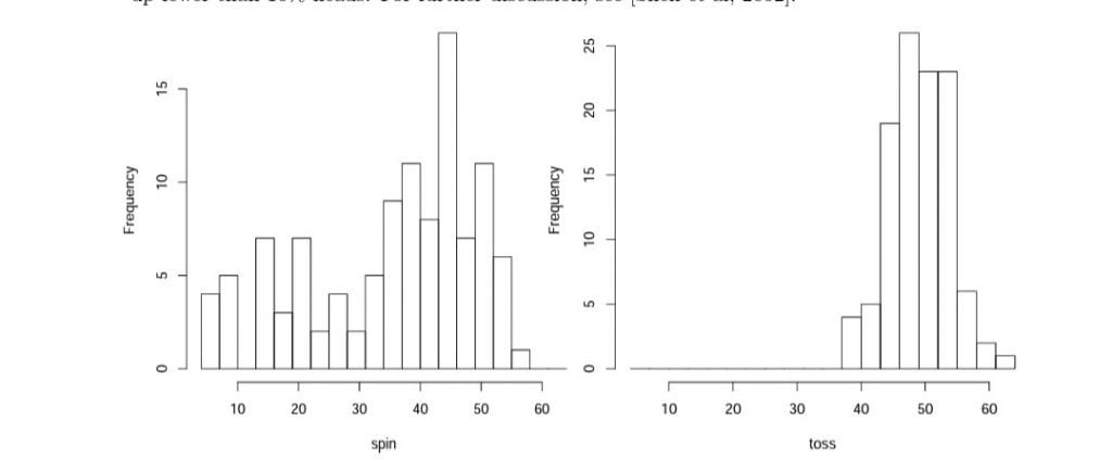
Priors Modified for Coin Tossing

Suppose, we have \(62\) heads in \(100\) tosses. The updated densities from our uniform, symmetric, and skewed priors doesn't show much difference. Bernoulli's inference from frequency to chance doesn't look too bad here, but now we know what assumptions we had to make to get that result.

There are limited number of shapes that can be made with beta priors. Now if one is aware of the technicalities of coin tossing, then one might want a different shape to quantify their state of prior ignorance. Persi Diaconis, a dedicated Bayesian and an experienced person regarding coin tossing, points out that coins spun on edge tend to be biased one way or another but more often towards tails. So, if an unknown coin is to be spun, Persi would prefer to put his beliefs on a bimodal prior density with somewhat higher peak on the tails' side, which can't be represented by beta distribution. However, we can represent such distributions, by mixtures of two beta densities, one peaked towards heads and one peaked towards tails, where the second peak is of higher altitude. Updating on frequency evidence is still relatively simple, treating the two betas as metahypotheses and their weights as prior probabilities.

More generally, one has a very high rich palette of shapes available for quantifying prior states of beliefs using finite mixtures of betas. Arguably one can get anything one might find rational to represent their prior mixture of knowledge and ignorance. As before, with lot of evidence such niceties will not matter much. But if we are going to risk a lot on the next few trials, it would be prudent for us to devote some thought to putting whatever we know into our prior.

Laplace continues...

Having his principle structured , he first applied his new, "probability of causes", to solve two gambling problems when he realized that his principle need more modification. In each case he understood intuitively what should happen but got bogged down trying to prove it mathematically. First problem, we worked with an urn filled with black and white tickets in an unknown proportion ( his cause). He first drew some number of tickets from the urn and based on that experience, asked for the probability that in the next draw his ticket will be white. To, prove the answer , he fought a frustrating battle and had to write \(45 \) equations, covering every corner of four quarto-sized pages. Today those \(45\) equations became redundant, or better to say reduced and compressed within of lines of simulation codes.

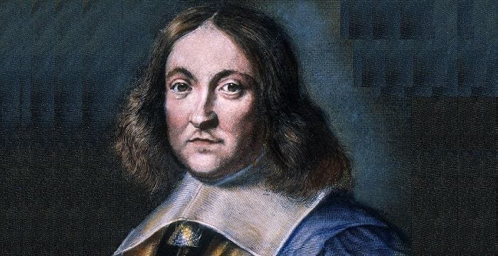
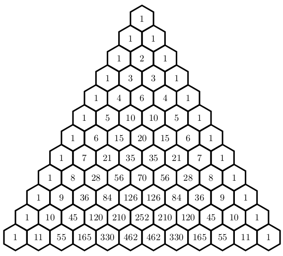
His second problem involved a piquet, a game requiring both luck and skill. Two people start playing but stop midway through the game and have to figure out how to divide the kitty by estimating their relative skill levels ( the cause). This problems, surely reminds us about the problems on which Pascal and Fermat worked, but there they both assumed that the players have equal skills. Laplace's version is more realistic.

With these two gambling problems, Laplace dealt with two very important perspective of uncertainties, first that is unknown parameter, first problem quite remarkably portrays the basic motive of Statistical Inference. And in the second problem, he dealt with even more finer perspective of uncertainty, that is Chance and Causes, which in future make this Bayes-Laplace model to be an important and comprehensive tool in drawing conclusion in the new Science of Cause and Effect.

Laplace, was then to move towards solving his actual problems in astronomy. How should they deal with different observations of the same phenomenon ? He was all set to address three of that era's biggest problems, that involved Gravitational attraction on the motions of our moon, the motions of the planets Jupiter and Saturn, and shape of the Earth. We shall keep the application of Bayesian Probabilities in these astronomical problems for some other day.

Laplace eventually credits Bayes

Eventhough, after the surfacing and developments of the Bayesian perspective, Statistical fraternity, got divided into the two groups of Frquentists and Bayesians, ironically, both Bayes and Laplace were neutral themselves. Bayes, even in his published essay, referred his dependencies on the frequencies while get an idea about his prior assumption, and never ignited the debate neither foresee such kind of debates in future.

Similarly Laplace, in his book on Probabilities, acknowledges the relative resemblances in his principle of Probability of Causes and frequency methods, which I tried putting light on, in the previous sections. He besides from being the resurrecting Bayes' rule, also invented the Central Limit Theorem, which is more kind of an Frequencist's tool than a Bayesians'.

When Laplace started grappling with his probability of causes, and attacking problems in celestial mechanics in 1781, Richard Price arrives Paris and informed them about the discovery of Bayes'. Laplace immediately latched onto Bayes' ingenious invention, the starting guess, and incorporated it into his own, earlier version of the probability of causes. Hence, he was now confident that he was on the right track in assuming the prior causes equally likely, and assured himself about the validity of his principle. Everytime he gets a new information he could use the answer from his last solution as the starting point for another calculation, That is he goes on successively. And by assuming all the prior causes equally likely, he could now formulate his principle into a law or a theorem. Though soon he was to realise about the shortcomings of his assumption of equally likely, and hence the need for generalizing, which we already talked about a bit under the section Laplace Generalizes.

Laplace later credited Bayes with being first when he wrote, "The theory whose principles I explained some years after,.... he accomplished in an acute and very ingenious, though slightly awkward, manner. "

Although Bayes originated the probability of causes, Laplace discovered the same on his own. When, Bayes' Essay eas published by his friend Price, Laplace was only 15. The approach and the principle both Bayes and Laplace developed are independent mathematically speaking. We will be discussing in more details the mathematical perspectives of both Laplace and Bayes in our coming articles.

Till then, stay safe, and keep finding the solutions for the Gambling Problems Laplace worked on, they no more need 45 equations to be solved nowadays !!

References

1. 1. Probability Theory- the logic of science - E.T.Jaynes
2. 2. A Philosophical Essay on Probabilities - Peirre-Simon Laplace
3. 3. The theory that would not Die- Sharon Bertsch Mcgrayne
4. 4. Ten Great Ideas About Chance- Skyrms, Diaconis

Some Previous Posts

• Bayes and the Billiard Table - Cheenta Probability Series
• Nonconglomerability and the Law of Total Probability - Cheenta Probability Series

This is the first of the many posts, that I will be writing on the evolution of Bayesian Thinking and Inverse Inferences, in Probability Theory, which actually changed Statistics from a tool of Data interpretation to Causal Science.

When the facts change, I change my opinion. What do you do, sir ?

-John Maynard Keynes

In the climax of our last discussion, I kept my discussion about the Jelly-bean example incomplete to begin here afresh. (If you haven't read that, you can read it before we start, here it is Judgements in a Fitful Realm | Cheenta Probability Series ). There we were actually talking about the instances, how evidences can exihibit chanciness in this uncertain world. Today we will discuss how we can update our beliefs or judgements ( Judgemental Probabilities), based on these uncertain evidences, provided we have observed a pattern in the occurrence of this so-called circumstantial evidences.

Or in more formal literature, it is referred as Inverse-Inference, as we will first observe some outcomes and then we will go deeper investigating the plausible explanations in terms of chances, so as to have some presumed idea about future outcomes . There arises two immediate questions,

• How does it helps in predicting or foresee future ?
• Why a causal explanation should depend on probabilities ?

Before discussing these questions, let us discuss about the structure and some ideas behind this way of Probability Analysis. I hope with some example, the reader will able to answer the above questions themselves, and eventually appreciate this particular school of thought which inspite of lot of controversies inspired independent fields of Statistics, which made statistics one of the most important knowledge of this century. Statistics doesn't remain just a mere tool of data interpreting but, is now capable of giving causal explanations to anything and everything, from questions like whether "Smoking Causes Cancer", or " What is the chance of having a Nuclear accident?".

A century earlier, asking this sort of questions to a statistician, was outrageous, as most of the statisticians ( very likely to be egoistic), would not admit their inability in answering these sorts, would say more likely " its not answerable, due to lack of evidences", or in other words implying, "in order to find the chance of a nuclear accident, you first need to organize a planned nuclear accident !!"

Bayes makes his Glorious Entry

In 1763, in an article, "Essays towards solving a Problem in Doctrine of Chances", as authored by Thomas Bayes, he put his ideas as,

"Given the number of times in which an unknown event happened or failed.

Required the chance that probability of its happening in a single trial lies somewhere between any two degrees of Probability that can be named. "

Its Strange, that what Bayes stated is so coinciding with the idea of conglomerability stated by De Fenetti nearly after 200years. This is where, I feel the evolution of probability theory is so perplexing, since often quite advanced ideas emerged earlier, and then there basic explanations were put in to words afterwards. And then, there are people who put these pieces of jigsaw puzzles in places, we will come back to this works later some other day.

As Bayes' gravestone suggests, he died in 1761 at the age of 59. After 2 years of his death, his friend Richard Price, published his Essay. Price communicated the essay, together with an introduction and an appendix by himself to the Royal Society, got it published in its Philosophical Transactions in 1763. Price, while referring to Bayes' idea writes,

".....he says that his design at first thinks of the subject of it was, to find out a method by which we might judge concerning the probability that an event has to happen, in given circumstances, upon the supposition that we know nothing concerning it but that, under the same circumstances, it has happened a certain number of times and failed a certain other number of times. "

Basically, Bayes was talking about a machinery which would find the predictive probability that something will happen, next time, from the past information. Bayes predecessors, even including Bernoulli and de Moivre, had reasoned from chances to frequency. Bayes gave a mathematical foundation for- inference from frequencies to chances.

Even though, with advancement of his theory, Bayes' rule found many useful application from Breaking Enigma, to answering whether, Smoking causes Cancer or many other sorts, Bayes himself was not motivated to put his ideas on paper for solving a practical problem, on the contrary what motivated Bayes, was a philosophical debate which demanded mathematical argument. To, me what Bayes' idea propagates is the sole uniformity and subjectivity of nature. In one way it makes us convince that we are by virtue dependent on chances, but on the other hand it suggest with every new information, we always have a scope of improving our ideas about the uncertainty, which seemed more uncertain, before that extra bit of information. It simply tells, that it all depends on some God damn Information.

Bayes sees the Light

An incendiary mix of religion and mathematics exploded over England in 1748, when the Scottish philosopher David Hume published an essay attacking some of fundamental narratives of organized religions. Hume believed that we can't be absolutely certain about anything that is based only on traditional beliefs, testimony, habitual relationships, or cause and effect.

As it happens, God was regarded as the First Cause of everything, Hume's skepticism about cause-and-effect relationships was especially unsettling. Hume claimed that there is always association between certain objects or event, and how they occur. Like the earlier discussion, we are likely to umbrella on a rainy day, so there is a strong association with the weather and your carrying of umbrella, but that doesn't any how implies your umbrella is the cause why it is cloudy out there, rather its the other way around. This was a pretty straight forward illustration, but as Hume illustrates more philosophically, that,

"....Being determined by the custom transfer the past to the future, in all our inferences; where the past has been entirely regular and uniform, we expect the event with the greatest assurance, and leave no room for any contrary supposition. But where different effects have been found to follow from causes, which are to appearance exactly similar, all these various effects must occur to the mind in transferring the past to the future, and enter into our consideration, when we determine the probability of the event. Though we give preference to that which has been found most usual, and believe that this effect will exist, we must not overlook the other effects, but must to each of them a particular wei9ght and authority, in proportion as we have found it to be more less frequent. "

What actually, Hume tried to claim is that, you are taking umbrella that also even doesn't imply, its rainy or cloudy even, it may happen that you will use the umbrella to protect yourself from the heat, it may be less likely ( for a given person), but still not at all unworthy of neglecting it completely. And most important, the "design of the world" does not prove the existence of a creator, an ultimate cause. Because we can seldom be certain that a particular cause will have a particular effect, we must be content with finding only probable causes and probable effects.

Even though, Hume's essay was not mathematically sound it had profound scientific food for Bayes to think over it and develop a mathematics to quantify such probabilities. Many mathematicians and scientists used to believe that the inexplicability of the laws of the Nature, proves the existence of God, their First Cause. As de Moivre put it in his "Doctrine of Chances" , calculations about natural events would eventually reveal the underlying order of the universe and its exquisite "Wisdom and Design".

The arguments, motivated Bayes, and he became keen to find ways to treat these thoughts mathematically. Sitting in that century, directly develop a probabilistic mathematics was quite difficult, as the idea of Probability was itself not very clear to the then Thinkers and Mathematicians. It was that era, when people would only understand Gambling, if you utter the word Chance. By that time, while spending his days in French Prison ( because he was a Protestant), De Moivre already had solved a gambling problem, when he worked out from cause-to-effect( like finding the chance of getting four aces in one poker hand). But still no-one ever thought of working a problem other way around, i.e. predict the causes, for an observed effect. Bayes, got in interested in questions as, what if a poker player deals himself four aces in each of the three consecutive hands ? What is the underlying chance (or cause) that his deck is loaded ?

As, Bayes himself kept his idea hidden until his fried Price, rediscovered it, it is very difficult to guess what exactly piqued Bayes' interest in the problem of inverse probability. Though he was aware of De Moivre's works, and getting interested in probability as it applied to gambling. Alternatively, it may also happen that, he was worried about the cause of Gravity, that Newton suggested, but Newton neither gave any Causal validation of Gravity , nor he talked about the truthfulness of his theory. Hence this also can be the possible reason, why he got interested in developing mathematical arguments, to predict the cause from observed effects. Finally Bayes' interest may have been stimulated by Hume's philosophical essay.

Crystallizing the essence of inverse probability problem in his mind, Bayes decided that his ai is to achieve the approximate chance of a future event, about which he knew nothing about except the pattern regarding its past occurrence. It is guessed that sometime sandwiched between 1746 and 1749, when he developed an ingenious solution. To reach the solution Bayes devised a thought experiment, which can be metaphorically referred as a 1700s version of a computer simulation. We will get to the problem, after discussing a bit about how Bayes, modified the frequency interpreting of probability.

Bayes Modifies

At the very beginning of the essay Bayes takes the liberty to modify the general frequency interpretation, and ended up defining conditional probability, and as it happens his definition of probability were actually remarkable anticipations of the judgemental coherence views, which were developed by likes of De Fenetti and Ramsay, years after. After defining what we call mutually set of mutually exclusive and exhaustive set of events, Bayes goes forward explaining probability as,

"The Probability of any event is the ratio between the value at which an expectation depending on the happening of the event ought to be computed, and the value of the thing expected upon its happening. "

Like a true probabilist, Bayes defined probability from a gambling point of view, talking about payoff as an outcome of each event. But we also can treat the result itself as the payoff or expected value as a result of certain events.

As we already discussed and I tried to make the point several time, that probability of any event can be interpreted as the weighted average of the judgemental probabilities ( conditional probabilities), which are obtained while observing some available evidences, and the weights of the so-defined mean are the probability of observing those evidences.

\(P(A)=P(A|E_1)P(E_1)+P(A|E_2)P(E_2)+........+P(A|E_n)P(E_n)\) ; here A is any event, which is depending on some set of Evidences, say \(E={E_1, E_2,.....,E_n}\).

Though very important restriction imposed by Bayes here is that, the set of possible evidences must be mutually exclusive and form an exhaustive set. i.e. \(E_1,E_2,....,E_n\) are mutually exclusive and exhaustive set.

This visualization of probability is important, once you enter the Bayesian regime. Moreover, even though frequency probability is our basic and primary understanding of probability, I find this interpretation of judgemental probabilities or sometimes also called Likelihoods( we will see later), more general model of probability, though a bit of abstraction associated, but that the true nature of an art, right ! And probability is an Art !

so, getting back to Bayes' definition of probability, mathematically speaking, If your total Judgement about an experiment (or gamble) is \(N\) (that is you put \(N\) unit on contract in case of gamble), and the there is an event \(e\), then the payoff from your investment of \(N\), you may expect from the occurrence of the event \(e\) is \(N.P(e)\), or

\(P(e)=\frac{ Expected \ value \ of \ out \ of \ N, \ if \ e }{N}\)

where, \(P(e)\) as the chance of the event \(e\). He completes his definition by claiming that "by Chance I mean Probability".

On basis of this definition, Bayes argues for the basic properties of probability, like additivity of disjoint probabilities in terms of additivity of expectations. But I choose not to elaborate here, as we already discussed about this in our last post and also in the post about Conglomerability. ( read this article, for more elaborate discussion Nonconglomerability and the Law of Total Probability || Cheenta Probability Series ).

Bayes goes on to establish the definition of conditional probability. He gives a separate treatment for the case where the conditioning event precedes the conditioned one and the case where the conditioning is subsequent to the conditioned one. The latter case is a bit perplexing as it is saying like some thing already happened, now we need to travel back the time and find what might have happened (behind the scene), such that it can explain our observation. But thats what Bayes claimed to find right !! So, here Bayes give a very interesting argument in his fourth proposition, where he invites us to consider an infinite number of trials determining the occurrence of the conditioning and conditioned events,

"If there be two subsequent events to be determined every day, and each day the probability of the 2nd is \(\frac{b}{N}\) and the probability of both \(\frac{P}{N}\), and I am to receive \(N\) if both events happen on the 1rst day on which the 2nd does ; I say, according to these considerations, the probability of my obtaining \(N\) is \(\frac{P}{b}\)....."

So, what Bayes says is on the first day either the condition happens- or if not he is facing the same wager as before :

"Likewise, if this coincident should not happen I have an expectation of being reinstated in my former circumstances."

This is to say, the Probability that a event occurring, when you already observed that another event has occurred already, is just the ratio of the Expectation of the coincidence ( that both the desired event and the event which occured happened) and the Expectation of the the event that has occurred. Some time this ratio is often referred as the likelihood of the desired event, while using it in the Bayesian Probability structure.

taking the gambling realm as Bayes, the probability of win on the supposition that \(E_2\) ( the second ) did not happen on the first day is just the original probability of a win. Let us assume unit stakes, so that expectation equals Probability, to simplify the exposition.

Then letting \(E_1\) be the first event and \(E_2\) the second , he argues as follows:

\(P(win)=P(win \ on \ day \ 1)+P(win \ later)\)

\(= P(E_1 \ and \ E_2)+P( not \ E_2)P(win)\)

\(=P(E_1 \ and \ E_2)+ (1-P(E_2))P(win)\)

\(P(win)=\frac{P(E_1 \ and \ E_2)}{P(E_2)}\).

This is what Bayes considered as the probability of \(E_1\) on the supposition \(E_2\) is taken as a corollary ( that is \(E_2\) has occurred or true ), but the exposition of the corollary contains an interesting twist, it goes like,

"Suppose after the expectation given me in foregoing proposition, and before it is all known whether the first event has happened or not, I should find that the second event has happened; from hence I can only infer that the event is determined on which my expectation depended, and have no reason to esteem the value of my expectation either greater or less than before. "

Here with expectation, he always means the odds of that particular event, and now I explained several times how probability can actually be interpreted as expectation, so I hope readers face no difficulty ( unfamiliarity may still exist) while going along with this kind of literature.

Now, Bayes gives a money-pump argument :

"For if I have reason to think it less, it would be reasonable to give something to be reinstated in my former circumstances, and this over and over again as I should be informed that the second event had happened, which is evidently absurd. "

He concludes explaining the opposite scenario as,

"And the like absurdity plainly follows if you say I ought to set a greater value on my expectation than before, for yhen it would be reasonable for me to refuse something if offered on the condition that I relinquish it, and be reinstated in my former circumstances...."

These arguments by Bayes gives two basic implications that, eventhough he didn't developed the sound mathematics of the nature of the probabilities he proposed, he had the idea of coherence and by extension conglomerability, which were yet to be put into mathematical literature.

Bayes in front of the Billiard Table, Finally !!

With conditional probability in hand, Bayes proceeds to the problem with which he begins the Essay. Suppose a coin, about whose bias we know nothing at all, has been flipped \(n\) times and has been heads \(m\) times. If \(x\) is the chance that coin comes up heads on a single toss, Bayes requires

\( P( x \ in \ [a,b] | m \ heads \ in \ n \ tosses) \) .

\(=\frac{P(x \ in \ [a,b] \ and \ m \ heads \ in \ n \ tosses)}{P(m \ heads \ in \ n \ tosses)}\).

To evaluate this, Bayes must assume something about the prior probability density over the chances. Prior probability density is the basically the prior (or initial) information about the desired unknown (here it is \(x\)), which he first assumes, and then he went on finding the required probability, which is called the posterior probability, based on the priors he assumed and the observations he made. So, basically he keeps updating his knowledge about the desired unknown starting with a mere information about the desired unknown (\(x\)). But the controversy arises where, he assumes the prior probability, or he makes an assumption about the prior information, that is the overall pattern on the nature of \(x\). We will come to these later, first express Bayes' final touches while completing the solution.

Now Bayes assumes a uniform prior density as the correct quantification of knowing nothing concerning it. Anticipating that this might prove controversial, as I mentioned above, and of course it has, he later offers a different justification in a scholium. On this basis, he applies Newton's calculus to get,

\(\frac{\int^b_a{n \choose m} x^m(1-x)^{n-m}\,dx}{\int^1_0{n \choose m}x^m(1-x)^{n-m}\,dx}\).

How are these to be solved? Bayes evaluates integral in the denominator by a geometrical trick. This is Bayes' "billiard table" argument.

Suppose we throw a red ball at random on a table and mark its distance from the leftmost side. Now then we toss \(n\) black balls one by one on the table, as shown in the figure.Lets call a ball that falls to the right of the red ball a head and one that falls to the left a tail. This corresponds to choosing a bias at random and flipping a coin of that bias \(n\) times. Now nothing hangs on the first ball being the red one. We could just throw \(n+1\) balls on the table and choose the one to be the red ball, the one to set bias, at random. But if we choose the leftmost ball to the red one, all is black balls count as heads and if we choose the right one to be the red ball, no black balls count as heads, and so forth. Thus the probability of \(m\) heads in \(n\) tosses is same for \(m=0,1,....,n\), hence the required probability must be \(\frac{1}{n+1}\). This is the value of the integral in the denominator. The integral in the numerator is harder and no such close form solution exists. Bayes however gives a way of approximating it too.

In scholium , Bayes uses his evaluation of the denominator to argue for his quantification of ignorance. He argues that, he knows nothing about the event except that there are \(n\) trials, he have no reason to think that it would succeed in some number of trials rather than another. Hence, he suggests that there is nothing wrong in taking

\(P(m \ heads \ in \ n \ tosses)=\frac{1}{n+1}\), as our quantification of ignorance about outcomes. The uniform prior, in fact follows from this - although Bayes did not have the proof !!

Priors to Posteriors- Journey Continues !

Once Bayes suggested a way of solving the inverse problem, of finding a bias of a coin given you observed a numbers of heads out of a number of tosses,

Or even extending the "billiard table" argument, suppose you are facing towards the wall and I threw the red ball and it stopped some where on the table, now you need to actually pin-point the position of the red ball, so I kept tossing each black ball (\(n\) times ) and noting whether the black ball is landing towards the left of the red ball or the right, now using this information about the black ball with respect to the randomly placed red ball, you can actually have the idea about the portion of the table where the red ball had stopped, right ! Bayes already answered that !!

Now say if you want to be more precise about the position of the red ball, so you requested me to throw another set of \(n\) balls, and repeat what I was doing. But now you have extra bit of information, that is you atleast know the possible portion of the red balls, from the posteriors, that Bayes calculated for you, so now you don't need to make the uniform assumption, whereas now you can you your newly acquired information, as your new prior and again update your posterior to an improved posterior probability about where on the damn table, your red ball rests.

So, this is where the genius of Bayes, takes probability to another level, using two most beautiful aspects of mathematics, that is inverse thinking and recursion.

We will get back into the next discussion, where we will be discussing about more example, the aftermath of the Bayesian introduction in the world of uncertainty, the man who did everything to give Bayesian Probability its firm footing, and obviously, "How to calculate the probability that the sun will rise tomorrow, given it has risen everyday for 5000years !!" .

Till then, stay safe, and keep finding the red ball on the billiard table, but don't turn around !!

References

1. 1. An Essay towards Solving a Problem in the Doctrine of Chances - Thomas Bayes
2. 2. The theory that would not Die- Sharon Bertsch Mcgrayne
3. 3. Ten Great Ideas About Chance- Skyrms, Diaconis